
Backpropagation (BP), short for Error Backward Propagation, is a fundamental algorithm used to train neural network models for graph embeddings.
The BP algorithm encompasses two main stages:
- Forward Propagation: Input data is fed into the input layer of the neural network or model. It then moves forward through one or more hidden layers before generating an output at the output layer.
- Backpropagation: The generated output is compared with the actual or expected value. Subsequently, the error is conveyed from the output layer through the hidden layers and back to the input layer. During this process, the weights of the model are adjusted using the gradient descent technique.
The iterative adjustment of weights forms the core of the training process of a neural network. We will illustrate this with a concrete example.
Preparations
Neural Network
A neural network typically consists of several key components: an input layer, one or more hidden layers, and an output layer. Below is a simple example of a neural network architecture:
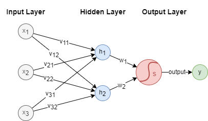
In this example, is the input vector with 3 features, and is the output. The hidden layer contains two neurons and , and the sigmoid activation function is applied at the output layer.
Furthermore, the connections between layers are characterized by weights: ~ connect the input layer to the hidden layer, while and connect the hidden layer to the output layer. These weights are pivotal in the computations performed within the neural network.
Activation Function
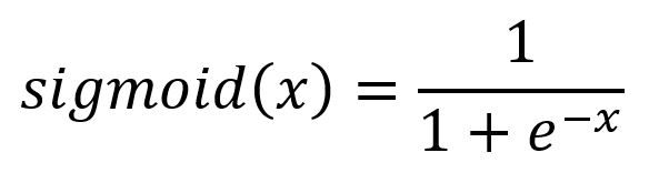
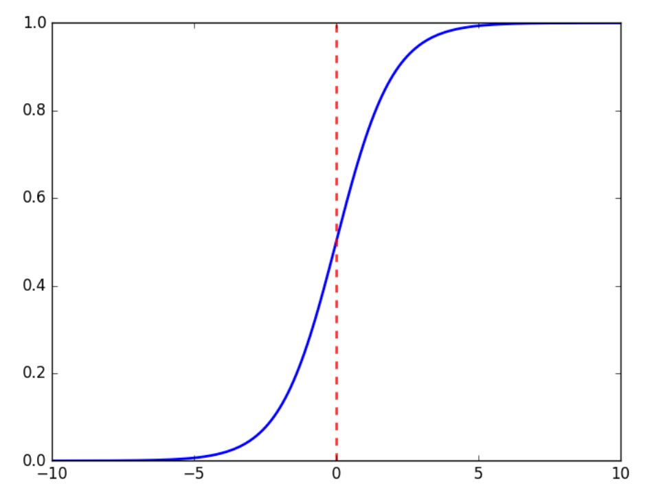
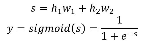
Activation functions enable neural networks to model non-linear relationships. Without them, the network can only represent linear mappings, which greatly limits its expressiveness. There are various activation functions available, each with its specific role. In this context, the sigmoid function is used, defined by the following formula and illustrated in the graph below:
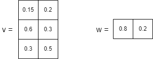
Initial Weights
The weights are initialized with random values. For illustration, let's assume the following initial weights:
Training Samples
Let's consider three sets of training samples, as shown below. The superscript indicates the order of the sample in the sequence:
- Inputs: , ,
- Outputs: , ,
The primary goal of the training process is to adjust the model's parameters (weights) so that the predicted/computed output () closely matches the actual output () when the input () is provided.
Forward Propagation
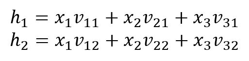
Input Layer → Hidden Layer
Neurons and are calculated by:
Hidden Layer → Output Layer
The output is calculated by:
Below is the calculation of the 3 samples:
| 2.4 | 1.8 | 2.28 | 0.907 | 0.64 | |
| 0.75 | 1.2 | 0.84 | 0.698 | 0.52 | |
| 1.35 | 1.4 | 1.36 | 0.796 | 0.36 |
Apparently, the three computed outputs () are very different from the expected ().
Backpropagation
Loss Function
A loss function is used to quantify the error or discrepancy between the model's predicted outputs and the expected outputs. It is also commonly referred to as the objective function or cost function. In this case, we'll use the mean squared error (MSE) as the loss function :
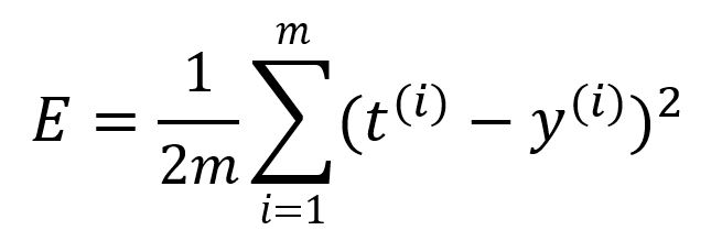
where is the number of samples. Calculate the error of this round of forward propagation as:
A smaller value of the loss function corresponds to higher model accuracy. The fundamental goal of model training is to minimize the value as much as possible.
By treating the inputs and outputs as constants and the weights as variables within the loss function, the goal becomes finding the weights that minimize the loss. This is precisely where the gradient descent technique comes into play.
In this example, batch gradient descent (BGD) is used, meaning all training samples are involved in the gradient calculation. The learning rate is set to .
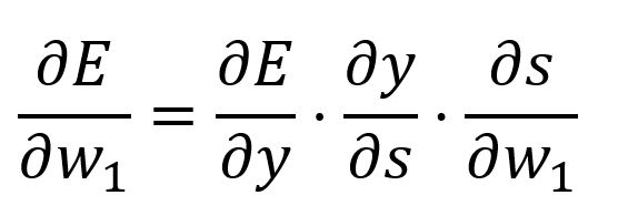
Output Layer → Hidden Layer
Adjust the weights and respectively.
Calculate the partial derivative of with respect to with the chain rule:
where,
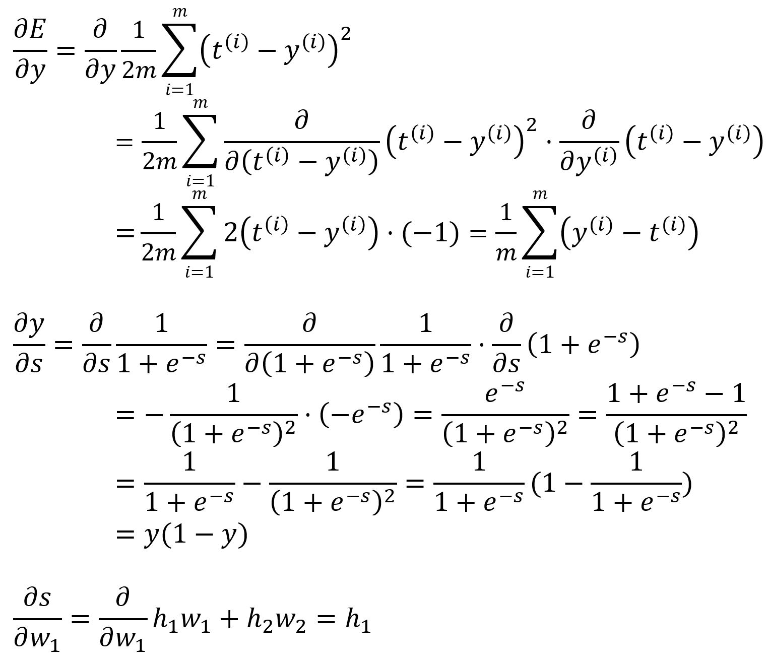
Calculate with values:
Then,
Since all samples are involved in computing the partial derivative, we calculate and by summing the derivatives across all samples and then taking the average.
Therefore, is updated to .
The weight can be updated in a similar way by calculating the partial derivative of with respect to . In this round, is updated from to .
Hidden Layer → Input Layer
Adjust the weights ~ respectively.
Calculate the partial derivative of with respect to with the chain rule:

We already computed and , below are the latter two:
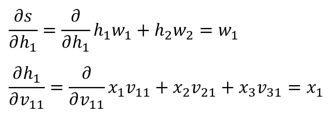
Calculate with values:
Then, .
Therefore, is updated to .
The remaining weights can be updated in a similar way by calculating the partial derivative of with respect to each weight. In this round, their values are updated as follows:
- is updated from to
- is updated from to
- is updated from to
- is updated from to
- is updated from to
Training Iterations
Apply the updated weights to the model and perform forward propagation again using the same three samples. In this iteration, the resulting error decreases to .
The backpropagation algorithm continues this cycle of forward and backward propagation iteratively to train the model. This process repeats until one of the following conditions is met: a predefined number of training iterations is completed, a time limit is reached, or the error falls below a specific threshold.