
Overview
The Louvain algorithm is a widely used and and well-regarded method for community detection in graphs. It is named after the location of its authors - Vincent D. Blondel et al. from Université catholique de Louvain in Belgium. The algorithm aims to maximize the modularity of the graph, and it has gained popularity due to its efficiency and the quality of its results.
- V.D. Blondel, J. Guillaume, R. Lambiotte, E. Lefebvre, Fast unfolding of communities in large networks (2008)
- H. Lu, Parallel Heuristics for Scalable Community Detection (2014)
Concepts
Modularity
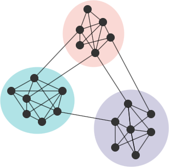
In many networks, nodes tend to naturally form groups or communities, characterized by dense connections within a community and relatively sparse connections between communities.
Consider an equivalent network G' to G, where G' remains the same community partition and the same number of edges as in G, but the edges are placed randomly. If G has a strong community structure, the ratio of intra-community edges to the total number of edges in G should be higher than the expected ratio in G'. A greater disparity between the actual ratio and expected ratios indicates a more prominent community structure in G. This concept forms the basis of modularity. The modularity is one of the widely used methods to evaluate the quality of a community partition. The Louvain algorithm is designed to find partitions that maximize modularity.
Modularity is a value that ranges from -1 to 1. A value close to 1 indicates a strong community structure, while negative values imply that the partitioning is likely not meaningful. For a connected graph, the modularity generally falls within the range of -0.5 to 1.
Considering the weights of edges in the graph, the modularity (Q) is defined as
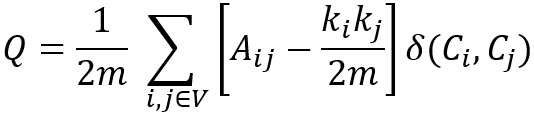
where,
- m is the total sum of edge weights in the graph;
- Aij is the sum of edge weights between nodes i and j, and 2m = ∑ijAij;
- ki is the sum of weights of all edges attached to node i;
- Ci represents the community to which node iis assigned, δ(Ci,Cj) is 1 if Ci= Cj, and 0 otherwise.
Note, is the expected sum of weights of edges between nodes i and j if edges are placed at random. Both Aij and are divided by 2m because each pair of distinct nodes in a community is considered twice, such as Aab = Aba, = .
We can also write the above formula as the following:
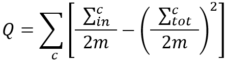
where,
- is the sum of weights of edges inside community C, i.e., the intra-community weight;
- is the sum of weights of edges incident to nodes in community C, i.e, the total-community weight;
- m has the same meaning as above, and 2m = ∑c.
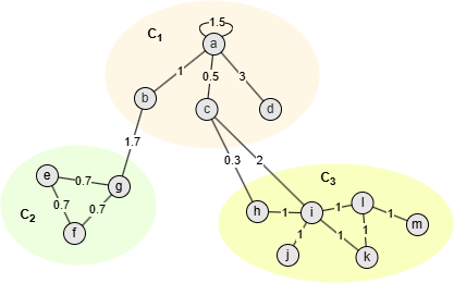
Nodes in this graph are assigned into 3 communities, take community C1 as example:
- = Aaa + Aab + Aac + Aad + Aba + Aca + Ada = 1.5 + 1 + 0.5 + 3 + 1 + 0.5 + 3 = 10.5
- ()2 = kaka + kakb + kakc + kakd + kbka + kbkb + kbkc + kbkd + kcka + kckb + kckc + kckd + kdka + kdkb + kdkc + kdkd + = (ka + kb + kc + kd)2 = (6 + 2.7 + 2.8 + 3)2 = 14.52
Louvain
The Louvain algorithm begins with a singleton partition, where each node belongs to its own community. It then proceeds iteratively through multiple passes, each consisting of two distinct phases.
First Phase: Modularity Optimization
For each node i, the algorithm considers all its neighbors j and calculates the gain of modularity (ΔQ) that would result from moving i from its current community to the community of j.
Node i is reassigned to the community that yields the maximum ΔQ, provided that this gain exceeds a predefined positive threshold. If no such gain is found, i remains in its original community.
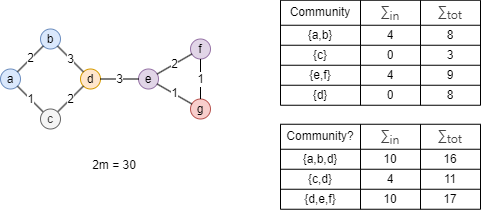
Take the graph above as an example, where nodes belonging to the same community are denoted with the same color. Now, consider node d. The modularity gains from moving it into the community {a,b}, {c}, and {e,f} are:
- ΔQd→{a,b} = Q{a,b,d} - (Q{a,b} + Q{d}) = 52/900
- ΔQd→{c} = Q{c,d} - (Q{c} + Q{d}) = 72/900
- ΔQd→{e,f} = Q{d,e,f} - (Q{e,f} + Q{d}) = 36/900
If ΔQd→{c} exceeds the predefined threshold of ΔQ, node d will be moved to community {c}; otherwise, it remains in its original community.
This process is applied sequentially to all nodes and repeated until no further individual move yields an improvement in modularity, or the maximum loop number is reached, completing the first phase.
Second Phase: Community Aggregation
In the second phase, each community is aggregated into a single node. Each of these aggregated nodes has a self-loop whose weight equals the total weight of intra-community edges. The weight of the edge between any two aggregated nodes corresponds to the sum of the weights of all edges between nodes in the respective original communities.
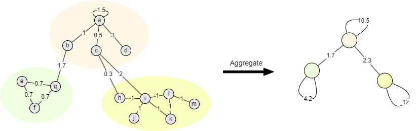
Community aggregation reduces the number of nodes and edges in the graph without altering local or global edge weights. After this compression, nodes within a community are treated as a single unit, allowing modularity optimization to continue at a higher level. This results in a hierarchical (iterative), multi-level community structure.
Once this second phase is completed, the algorithm applies another pass on the aggregated graph. hese passes repeat iteratively until no further modularity gains can be achieved, at which point the final community structure is established.
Considerations
- If node i has any self-loop, when calculating ki, the weight of self-loop is counted only once.
- The Louvain algorithm treats all edges as undirected, ignoring their original direction.
- The output of the Louvain algorithm may vary across executions due to the order in which nodes are processed. However, this variation typically has little impact on the final modularity value.
Example Graph
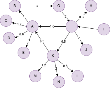
Run the following statements on an empty graph to define its structure and insert data:
ALTER EDGE default ADD PROPERTY {
    weight float
};
INSERT (A:default {_id: "A"}),
       (B:default {_id: "B"}),
       (C:default {_id: "C"}),
       (D:default {_id: "D"}),
       (E:default {_id: "E"}),
       (F:default {_id: "F"}),
       (G:default {_id: "G"}),
       (H:default {_id: "H"}),
       (I:default {_id: "I"}),
       (J:default {_id: "J"}),
       (K:default {_id: "K"}),
       (L:default {_id: "L"}),
       (M:default {_id: "M"}),
       (N:default {_id: "N"}),
       (A)-[:default {weight: 1}]->(B),
       (A)-[:default {weight: 1.7}]->(C),
       (A)-[:default {weight: 0.6}]->(D),
       (A)-[:default {weight: 1}]->(E),
       (B)-[:default {weight: 3}]->(G),
       (F)-[:default {weight: 1.6}]->(A),
       (F)-[:default {weight: 0.3}]->(H),
       (F)-[:default {weight: 2}]->(J),
       (F)-[:default {weight: 0.5}]->(K),
       (G)-[:default {weight: 2}]->(F),
       (I)-[:default {weight: 1}]->(F),
       (K)-[:default {weight: 0.3}]->(A),
       (K)-[:default {weight: 0.8}]->(L),
       (K)-[:default {weight: 1.2}]->(M),
       (K)-[:default {weight: 2}]->(N);
create().edge_property(@default, "weight", float);
insert().into(@default).nodes([{_id:"A"}, {_id:"B"}, {_id:"C"}, {_id:"D"}, {_id:"E"}, {_id:"F"}, {_id:"G"}, {_id:"H"},{_id:"I"},{_id:"J"},{_id:"K"},{_id:"L"},{_id:"M"},{_id:"N"}]);
insert().into(@default).edges([{_from:"A", _to:"B", weight:1}, {_from:"A", _to:"C", weight:1.7}, {_from:"A", _to:"D", weight:0.6}, {_from:"A", _to:"E", weight:1}, {_from:"B", _to:"G", weight:3}, {_from:"F", _to:"A", weight:1.6}, {_from:"F", _to:"H", weight:0.3}, {_from:"F", _to:"J", weight:2}, {_from:"F", _to:"K", weight:0.5}, {_from:"G", _to:"F", weight:2}, {_from:"I", _to:"F", weight:1}, {_from:"K", _to:"A", weight:0.3}, {_from:"K", _to:"M", weight:1.2}, {_from:"K", _to:"N", weight:2}, {_from:"K", _to:"L", weight:0.8}]);
Creating HDC Graph
To load the entire graph to the HDC server hdc-server-1 as my_hdc_graph:
CREATE HDC GRAPH my_hdc_graph ON "hdc-server-1" OPTIONS {
  nodes: {"*": ["*"]},
  edges: {"*": ["*"]},
  direction: "undirected",
  load_id: true,
  update: "static"
}
hdc.graph.create("my_hdc_graph", {
  nodes: {"*": ["*"]},
  edges: {"*": ["*"]},
  direction: "undirected",
  load_id: true,
  update: "static"
}).to("hdc-server-1")
Parameters
Algorithm name: louvain
Name |
Type |
Spec |
Default |
Optional |
Description |
|---|---|---|---|---|---|
phase1_loop_num |
Integer | ≥1 | 5 |
Yes | The maximum number of loops in the first phase during each pass. |
min_modularity_increase |
Float | [0,1] | 0.01 |
Yes | The minimum gain of modularity (ΔQ) to move a node to another community. |
edge_schema_property |
[]"<@schema.?><property>" |
/ | / | Yes | Numeric edge properties used as weights, summing values across the specified properties; edges without this property are ignored. |
return_id_uuid |
String | uuid, id, both |
uuid |
Yes | Includes _uuid, _id, or both to represent nodes in the results. |
limit |
Integer | ≥-1 | -1 |
Yes | Limits the number of results returned. Set to -1 to include all results. |
order |
String | asc, desc |
/ | Yes | Sorts the results by count; this option is only valid in Stream Return when mode is set to 2. |
File Writeback
This algorithm can generate three files:
Spec |
Content |
|---|---|
filename_community_id |
|
filename_ids |
|
filename_num |
|
CALL algo.louvain.write("my_hdc_graph", {
  return_id_uuid: "id",
  phase1_loop_num: 5,
  min_modularity_increase: 0.1,
  edge_schema_property: 'weight'
}, {
  file: {
    filename_community_id: "f1",
    filename_ids: "f2",
    filename_num: "f3"
  }
})
algo(louvain).params({
  projection: "my_hdc_graph",
  return_id_uuid: "id",
  phase1_loop_num: 5,
  min_modularity_increase: 0.1,
  edge_schema_property: 'weight'
}).write({
  file: {
    filename_community_id: "f1",
    filename_ids: "f2",
    filename_num: "f3"
  }
})
Result:
_id,community_id
I,5
G,7
J,5
D,13
N,11
F,5
H,5
B,7
L,11
A,13
E,13
K,11
M,11
C,13
community_id,_ids
13,D;A;E;C;
5,I;J;F;H;
7,G;B;
11,N;L;K;M;
community_id,count
13,4
5,4
7,2
11,4
DB Writeback
Writes the community_id values from the results to the specified node property. The property type is uint32.
CALL algo.louvain.write("my_hdc_graph", {
  return_id_uuid: "id",
  phase1_loop_num: 5,
  min_modularity_increase: 0.1,
  edge_schema_property: 'weight'
}, {
  db: {
    property: "communityID"
  }
})
algo(louvain).params({
  projection: "my_hdc_graph",
  return_id_uuid: "id",
  phase1_loop_num: 5,
  min_modularity_increase: 0.1,
  edge_schema_property: 'weight'
}).write({
  db: {
    property: 'communityID'
  }
})
Stats Writeback
CALL algo.louvain.write("my_hdc_graph", {
  return_id_uuid: "id",
  phase1_loop_num: 5,
  min_modularity_increase: 0.1,
  edge_schema_property: 'weight'
}, {
  stats: {}
})
algo(louvain).params({
  projection: "my_hdc_graph",
  return_id_uuid: "id",
  phase1_loop_num: 5,
  min_modularity_increase: 0.1,
  edge_schema_property: 'weight'
}).write({
  stats: {}
})
Result:
| community_count | modularity |
|---|---|
| 4 | 0.464280 |
Full Return
CALL algo.louvain.run("my_hdc_graph", {
  return_id_uuid: "id",
  phase1_loop_num: 5,
  min_modularity_increase: 0.1
}) YIELD r
RETURN r
exec{
  algo(louvain).params({
    return_id_uuid: "id",
    phase1_loop_num: 5,
    min_modularity_increase: 0.1
  }) as r
  return r
} on my_hdc_graph
Result:
| _id | community_id |
|---|---|
| I | 5 |
| G | 7 |
| J | 5 |
| D | 9 |
| N | 11 |
| F | 5 |
| H | 5 |
| B | 7 |
| L | 11 |
| A | 9 |
| E | 9 |
| K | 11 |
| M | 11 |
| C | 9 |
Stream Return
This Stream Return supports two modes:
| Item | Spec | Columns |
|---|---|---|
mode |
1 (Default) |
|
2 |
|
CALL algo.louvain.stream("my_hdc_graph", {
  return_id_uuid: "id",
  phase1_loop_num: 6,
  min_modularity_increase: 0.1
}) YIELD r
RETURN r
exec{
  algo(louvain).params({
    return_id_uuid: "id",
    phase1_loop_num: 6,
    min_modularity_increase: 0.1
  }).stream() as r
  return r
} on my_hdc_graph
Result:
| _id | community_id |
|---|---|
| I | 5 |
| G | 7 |
| J | 5 |
| D | 9 |
| N | 11 |
| F | 5 |
| H | 5 |
| B | 7 |
| L | 11 |
| A | 9 |
| E | 9 |
| K | 11 |
| M | 11 |
| C | 9 |
CALL algo.louvain.stream("my_hdc_graph", {
  return_id_uuid: "id",
  phase1_loop_num: 6,
  min_modularity_increase: 0.1,
  order: "asc"
}, {
  mode: 2
}) YIELD r
RETURN r
exec{
  algo(louvain).params({
    return_id_uuid: "id",
    phase1_loop_num: 6,
    min_modularity_increase: 0.1,
    order: "asc"
  }).stream({
    mode: 2
  }) as r
  return r
} on my_hdc_graph
Result:
| community_id | count |
|---|---|
| 7 | 2 |
| 5 | 4 |
| 9 | 4 |
| 11 | 4 |
Stats Return
CALL algo.louvain.stats("my_hdc_graph", {
  return_id_uuid: "id",
  phase1_loop_num: 6,
  min_modularity_increase: 0.1
}) YIELD s
RETURN s
exec{
  algo(louvain).params({
    return_id_uuid: "id",
    phase1_loop_num: 6,
    min_modularity_increase: 0.1
  }).stats() as s
  return s
} on my_hdc_graph
Result:
| community_count | modularity |
|---|---|
| 4 | 0.397778 |
Algorithm Efficiency
The Louvain algorithm achieves lower time complexity than previous community detection algorithms through its improved greedy optimization, which is usually regarded as O(N*logN), where N is the number of nodes in the graph, and the result is more intuitive. For instance, in a graph with 10,000 nodes, the complexity of the Louvain algorithm is around O(40000); in a connected graph with 100 million nodes, the algorithm complexity is around O(800000000).
However, upon closer inspection of the algorithm process breakdown, we can see that the complexity of the Louvain algorithm depends not only on the number of nodes but also on the number of edges. Roughly speaking, it can be approximated as O(N * E/N) = O(E), where E is the number of edges in the graph. This is because the dominant algorithm logic of Louvain is to calculate the weights of edges attached to each node.
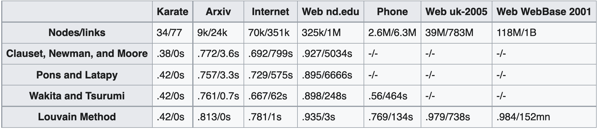
The table below shows the performance of the community detection algorithms of Clauset, Newman and Moore, of Pons and Latapy, of Wakita and Tsurumi, and Louvain, in networks of various sizes. For each algorithm/network, it gives the modularity that is gained and the computation time. Empty record indicates a computation time that is over 24 hours. It clearly demonstrates that Louvain achieves a significant (exponential) increase in both modularity and efficiency.
The choice of system architecture and programming language can significantly impact the efficiency and final results of the Louvain algorithm. For example, a serial implementation of the Louvain algorithm in Python may result in hours of computation time for small graphs with around 10,000 nodes. Additionally, the data structure used can influence performance, as the algorithm frequently calculates node degrees and edge weights.
The native Louvain algorithm adopts C++, but it is a serial implementation. The time consumption can be reduced by using parallel computation as much as possible, thereby improving the efficiency of the algorithm.
For medium-sized graphset with tens of millions of nodes and edges, Ultipa's Louvain algorithm can be completed literally in real time. For large graphs with over 100 million nodes and edges, it can be implemented in seconds to minutes. Furthermore, the efficiency of the Louvain algorithm can be affected by other factors, such as whether data is written back to the database property or disk file. These operations can impact the overall computation time of the algorithm.
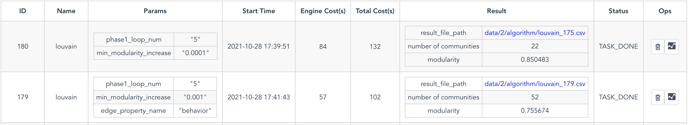
This is the records of the modularity and execution time of the Louvain algorithm running on a graph with 5 million nodes and 100 million edges. The computation process takes approximately 1 minute, and additional operations, such as writing back to the database or generating a disk file, add around 1 minute to the total execution time.