
Overview
LINE (Large-scale Information Network Embedding) is a network embedding model that preserves the local or global network structures. LINE is able to scale to very large, arbitrary types of networks, it was originally proposed in 2015:
- J. Tang, M. Qu, M. Wang, M. Zhang, J. Yan, Q. Zhu, LINE: Large-scale Information Network Embedding (2015)
Concepts
First-order Proximity and Second-order Proximity
First-order proximity in a network shows the local proximity between two nodes, and it is contingent upon connectivity. The existence of a link or a link with a larger weight (negative weight is not considered here) signifies greater first-order proximity among two nodes; if no link exist in-between, their first-order proximity is 0.
On the other hand, second-order proximity between a pair of nodes is the similarity between their neighborhood structure, which is determined through the shared neighbors. In case two nodes lack common neighbors, their second-order proximity is 0.
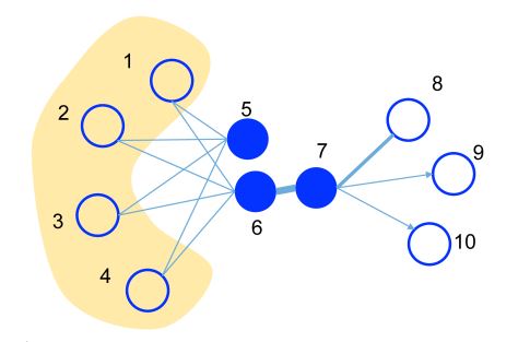
This is an illustrative example, where the edge thickness signifies its weight.
- A substantial weight on the edge between nodes 6 and 7 indicates a high first-order proximity. They shall have close representations in the embedding space.
- Though nodes 5 and 6 are not directly connected, their considerable common neighbors establish a notable second-order proximity. They are expected to be represented closely to each other in the embedding space as well.
LINE Model
The LINE model is designed to embed nodes in graph G = (V,E) into low-dimensional vectors, preserving the first- or second-order proximity between nodes.
LINE with First-order Proximity
To capture the first-order proximity, LINE defines the joint probability for each edge (i,j)∈E connecting nodes vi and vj as follows:
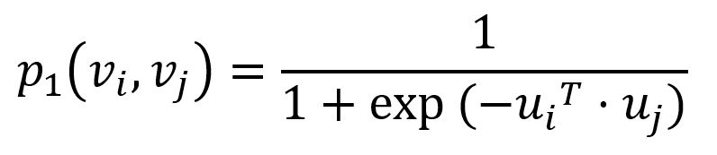
where ui is the low-dimensional vector representation of node vi. The joint probability p1 ranges from 0 to 1, with two closer vectors resulting in a higher dot product and, consequently a higher joint probability.
Empirically, the joint probability between node vi and vj can be defined as
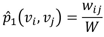
where wij denotes the edge weight between nodes vi and vj, W is the sum of all edge weights in the graph.
The KL-divergence is adopted to measure the difference between two distributions:
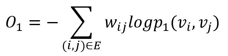
This serves as the objective function that needs to be minimized during training when preserving the first-order proximity.
LINE with Second-order Proximity
To model the second-order proximity, LINE defines two roles for each node - one as the node itself, another as "context" for other nodes (this concept originates from the Skip-gram model). Accordingly, two vector representations are introduced for each node.
For each edge (i,j)∈E, LINE defines the probability of "context" vj be observed by node vi as
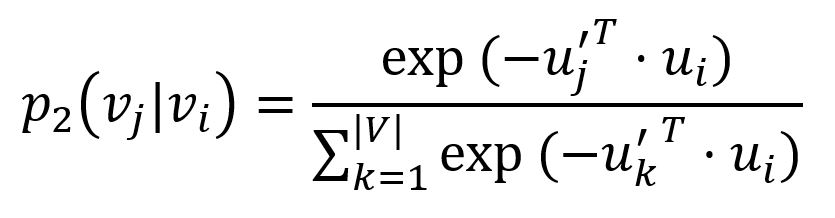
where u'j is the representation of node vj when it is regarded as the "context". Importantly, the denominator involves the whole "context" in the graph.
The corresponding empirical probability can be defined as
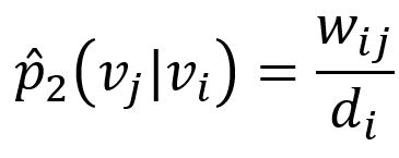
where wij is weight of edge (i,j), di is the weighted degree of node vi.
Similarly, the KL-divergence is adopted to measure the difference between two distributions:
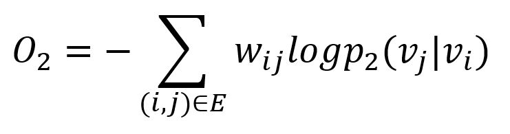
This serves as the objective function that needs to be minimized during training when preserving the second-order proximity.
Model Optimization
Negative Sampling
To improve the computation efficiency, LINE adopts the negative sampling approach which samples multiple negative edges according to some noisy distribution for each edge (i,j). Specifically, the two objective functions are adjusted as:
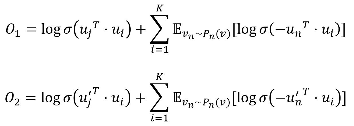
where σ is the sigmoid function, K is the number of negative edges drawn from the noise distribution Pn(v) ∝ dv3/4, dv is the weighted degree of node v.
Edge-Sampling
Since the edge weights are included in both objectives, these weights will be multiplied into gradients, resulting in the explosion of the gradients and thus compromise the performance. To address this, LINE samples the edges with the probabilities proportional to their weights, and then treat the sampled edges as binary edges for model updating.
Considerations
- The LINE algorithm ignores the direction of edges but calculates them as undirected edges.
Example Graph
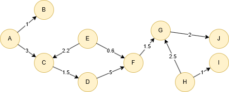
To create this graph:
// Runs each row separately in order in an empty graphset
create().edge_property(@default, "score", float)
insert().into(@default).nodes([{_id:"A"},{_id:"B"},{_id:"C"},{_id:"D"},{_id:"E"},{_id:"F"},{_id:"G"},{_id:"H"},{_id:"I"},{_id:"J"}])
insert().into(@default).edges([{_from:"A", _to:"B", score:1}, {_from:"A", _to:"C", score:3}, {_from:"C", _to:"D", score:1.5}, {_from:"D", _to:"F", score:5}, {_from:"E", _to:"C", score:2.2}, {_from:"E", _to:"F", score:0.6}, {_from:"F", _to:"G", score:1.5}, {_from:"G", _to:"J", score:2}, {_from:"H", _to:"G", score:2.5}, {_from:"H", _to:"I", score:1}])
Creating HDC Graph
To load the entire graph to the HDC server hdc-server-1 as hdc_line:
CALL hdc.graph.create("hdc-server-1", "hdc_line", {
  nodes: {"*": ["*"]},
  edges: {"*": ["*"]},
  direction: "undirected",
  load_id: true,
  update: "static",
  query: "query",
  default: false
})
hdc.graph.create("hdc_line", {
  nodes: {"*": ["*"]},
  edges: {"*": ["*"]},
  direction: "undirected",
  load_id: true,
  update: "static",
  query: "query",
  default: false
}).to("hdc-server-1")
Parameters
Algorithm name: line
Name |
Type |
Spec |
Default |
Optional |
Description |
|---|---|---|---|---|---|
edge_schema_property |
[]"@<schema>?.<property>" |
/ | / | No | Numeric edge properties used as edge weights, summing values across the specified properties; edges without the specified properties are ignored. |
dimension |
Integer | ≥2 | / | No | Dimensionality of the embeddings. |
train_total_num |
Integer | ≥1 | / | No | Total number of training iterations. |
train_order |
Integer | 1, 2 |
1 |
Yes | Type of proximity to preserve, 1 means first-order proximity, 2 means second-order proximity. |
learning_rate |
Float | (0,1) | / | No | Learning rate used initially for training the model, which decreases after each training iteration until reaches min_learning_rate. |
min_learning_rate |
Float | (0,learning_rate) |
/ | No | Minimum threshold for the learning rate as it is gradually reduced during the training. |
neg_num |
Integer | ≥1 | / | Yes | Number of negative samples to produce for each positive sample, it is suggested to set between 1 to 10. |
resolution |
Integer | ≥1 | 1 |
Yes | The parameter used to enhance negative sampling efficiency; a higher value offers a better approximation to the original noise distribution; it is suggested to set as 10, 100, etc. |
return_id_uuid |
String | uuid, id, both |
uuid |
Yes | Includes _uuid, _id, or both values to represent nodes in the results. |
limit |
Integer | ≥-1 | -1 |
Yes | Limits the number of results returned; -1 includes all results. |
File Writeback
CALL algo.line.write("hdc_line", {
  params: {
    return_id_uuid: "id",
    edge_schema_property: "score",
    dimension: 3,
    train_total_num: 10,
    train_order: 1,
    learning_rate: 0.01,
    min_learning_rate: 0.0001,
    neg_number: 5,
    resolution: 100
  },
  return_params: {
    file: {
      filename: "embeddings"
    }
  }
})
algo(line).params({
  projection: "hdc_line",
  return_id_uuid: "id",
  edge_schema_property: "score",
  dimension: 3,
  train_total_num: 10,
  train_order: 1,
  learning_rate: 0.01,
  min_learning_rate: 0.0001,
  neg_number: 5,
  resolution: 100
}).write({
  file:{
    filename: 'embeddings'
  }
})
_id,embedding_result
J,0.134156,0.147224,-0.127542,
D,-0.110004,0.0445883,0.101143,
F,0.0306388,0.00733918,-0.11945,
H,0.0739559,-0.145214,0.0416526,
B,-0.02514,-0.0317756,-0.110371,
A,-0.0629673,0.0857267,0.100926,
E,0.0989685,0.0532481,0.0514933,
C,-0.127659,-0.136062,0.166552,
I,0.126709,0.103002,-0.0201314,
G,0.134589,-0.0157018,0.0237946,
DB Writeback
Writes the embedding_result values from the results to the specified node property. The property type is float[].
CALL algo.line.write("hdc_line", {
  params: {
    return_id_uuid: "id",
    edge_schema_property: "score",
    dimension: 3,
    train_total_num: 10,
    train_order: 1,
    learning_rate: 0.01,
    min_learning_rate: 0.0001,
    neg_number: 5,
    resolution: 100
  },
  return_params: {
    db: {
      property: "vector"
    }
  }
})
algo(line).params({
  projection: "hdc_line",
  return_id_uuid: "id",
  edge_schema_property: "score",
  dimension: 3,
  train_total_num: 10,
  train_order: 1,
  learning_rate: 0.01,
  min_learning_rate: 0.0001,
  neg_number: 5,
  resolution: 100
}).write({
  db: {
      property: "vector"
    }
})
Full Return
CALL algo.line("hdc_line", {
  params: {
    return_id_uuid: "id",
    edge_schema_property: '@default.score',
    dimension: 4,
    train_total_num: 10,
    train_order: 1,
    learning_rate: 0.01,
    min_learning_rate: 0.0001
  },
  return_params: {}
}) YIELD embeddings
RETURN embeddings
exec{
  algo(line).params({
    return_id_uuid: "id",
    edge_schema_property: '@default.score',
    dimension: 4,
    train_total_num: 10,
    train_order: 1,
    learning_rate: 0.01,
    min_learning_rate: 0.0001
  }) as embeddings
  return embeddings
} on hdc_line
Result:
_id |
embedding_result |
|---|---|
| J | [0.10039449483156204,0.11040361225605011,-0.095774807035923,-0.0819125771522522] |
| D | [0.0338507741689682,0.07575879991054535,0.023179633542895317,0.005116916261613369] |
| F | [-0.08940199762582779,0.05569583922624588,-0.10888427495956421,0.03145558759570122] |
| H | [-0.018580902367830276,-0.024093549698591232,-0.08332693576812744,-0.04651310294866562] |
| B | [0.0645807683467865,0.07539491355419159,0.07396885752677917,0.040248531848192215] |
| A | [0.03878217190504074,-0.09487584978342056,-0.10220742225646973,0.12434131652116776] |
| E | [0.09489674866199493,0.07733562588691711,-0.015262083150446415,0.10043458640575409] |
| C | [-0.01225052960216999,0.018636001273989677,-0.0036492166109383106,-0.0745576024055481] |
| I | [0.0327218696475029,-0.033543504774570465,-0.09600748121738434,0.11864277720451355] |
| G | [0.1094101220369339,-0.02683556079864502,-0.006420814897865057,0.012586096301674843] |
Stream Return
CALL algo.line("hdc_line", {
  params: {
    return_id_uuid: "id",
    edge_schema_property: '@default.score',
    dimension: 3,
    train_total_num: 10,
    train_order: 1,
    learning_rate: 0.01,
    min_learning_rate: 0.0001
  },
  return_params: {
  stream: {}}
}) YIELD embeddings
RETURN embeddings
exec{
  algo(line).params({
    return_id_uuid: "id",
    edge_schema_property: '@default.score',
    dimension: 3,
    train_total_num: 10,
    train_order: 1,
    learning_rate: 0.01,
    min_learning_rate: 0.0001
  }).stream() as embeddings
  return embeddings
} on hdc_line
Result:
_id |
embedding_result |
|---|---|
| J | [0.13375547528266907,0.14727242290973663,-0.12761451303958893] |
| D | [-0.10898537188768387,0.045617908239364624,0.09961149096488953] |
| F | [0.030374202877283096,0.0074587357230484486,-0.11920187622308731] |
| H | [0.0746561735868454,-0.1447625607252121,0.04158430173993111] |
| B | [-0.02504475973546505,-0.0319061279296875,-0.1105244979262352] |
| A | [-0.0629904493689537,0.08570709079504013,0.1011749655008316] |
| E | [0.09852229058742523,0.0527675524353981,0.05207677558064461] |
| C | [-0.1265311986207962,-0.1361672431230545,0.16603653132915497] |
| I | [0.12704375386238098,0.10234453529119492,-0.0199428740888834] |
| G | [0.1342623233795166,-0.016277270391583443,0.0242084339261055] |