Modularity
Overview
The Modularity algorithm evaluates the quality of an existing community partition by computing its modularity score. Unlike community detection algorithms that find communities, this algorithm measures how good a given partition is.
It is typically used after running a community detection algorithm (such as Louvain and Leiden) to assess the quality of the detected communities.
Concepts
Modularity
In many networks, nodes tend to naturally form groups or communities, characterized by dense connections within a community and relatively sparse connections between communities.
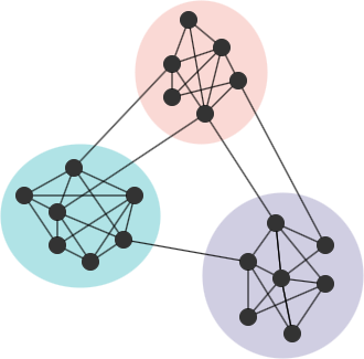
Consider an equivalent network G' to G, where G' remains the same community partition and the same number of edges as in G, but the edges are placed randomly. If G has a strong community structure, the ratio of intra-community edges to the total number of edges in G should be higher than the expected ratio in G'. A greater disparity between the actual ratio and expected ratios indicates a more prominent community structure in G. This concept forms the basis of modularity. The modularity is one of the widely used methods to evaluate the quality of a community partition. The Louvain algorithm is designed to find partitions that maximize modularity.
Modularity is a value that ranges from -1 to 1. A value close to 1 indicates a strong community structure, while negative values imply that the partitioning is likely not meaningful. For a connected graph, the modularity generally falls within the range of -0.5 to 1.
Considering the weights of edges in the graph, the modularity (Q) is defined as
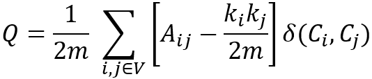
where,
mis the total sum of edge weights in the graph;Aijis the sum of edge weights between nodesiandj, and2m = ∑ijAij;kiis the sum of weights of all edges attached to nodei;Cirepresents the community to which node iis assigned,δ(Ci,Cj)is 1 ifCi= Cj, and 0 otherwise.
Note, is the expected sum of weights of edges between nodes i and j if edges are placed at random. Both Aij and are divided by 2m because each pair of distinct nodes in a community is considered twice, such as Aab = Aba, = .
We can also write the above formula as the following:
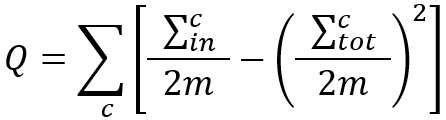
where,
is the sum of weights of edges inside communityC, i.e., the intra-community weight;is the sum of weights of edges incident to nodes in communityC, i.e, the total-community weight;mhas the same meaning as above, and2m = ∑c.
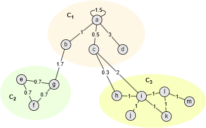
Nodes in this graph are assigned into 3 communities, take community C1 as example:
- = Aaa + Aab + Aac + Aad + Aba + Aca + Ada = 1.5 + 1 + 0.5 + 3 + 1 + 0.5 + 3 = 10.5
- ()2 = kaka + kakb + kakc + kakd + kbka + kbkb + kbkc + kbkd + kcka + kckb + kckc + kckd + kdka + kdkb + kdkc + kdkd + = (ka + kb + kc + kd)2 = (6 + 2.7 + 2.8 + 3)2 = 14.52
Considerations
- The algorithm treats all edges as undirected.
- Community assignments are read from a node property specified by
communityProperty. If not specified, each node is treated as its own community.
Example Graph

GQLINSERT (A:default {_id: "A", comm_id: 0}), (B:default {_id: "B", comm_id: 0}),
       (C:default {_id: "C", comm_id: 0}), (D:default {_id: "D", comm_id: 1}),
       (E:default {_id: "E", comm_id: 1}), (F:default {_id: "F", comm_id: 1}),
       (G:default {_id: "G", comm_id: 2}), (H:default {_id: "H", comm_id: 2}),
       (A)-[:default]->(B), (A)-[:default]->(C),
       (B)-[:default]->(C), (A)-[:default]->(D),
       (D)-[:default]->(E), (D)-[:default]->(F),
       (E)-[:default]->(F), (G)-[:default]->(D),
       (G)-[:default]->(H)
Parameters
| Name | Type | Default | Description |
|---|---|---|---|
communityProperty | STRING | / | Node property storing community assignments. If not specified, each node is treated as its own community. |
Run Mode
Returns:
| Column | Type | Description |
|---|---|---|
modularity | FLOAT | Overall modularity score Q |
communityCount | INT | Number of communities |
GQLCALL algo.modularity({
  communityProperty: "comm_id"
}) YIELD modularity, communityCount
Stream Mode
Returns the same columns as run mode, streamed for memory efficiency.
GQLCALL algo.modularity.stream({
  communityProperty: "comm_id"
}) YIELD modularity, communityCount
RETURN modularity, communityCount
Stats Mode
Returns:
| Column | Type | Description |
|---|---|---|
nodeCount | INT | Total number of nodes |
modularity | FLOAT | Overall modularity score Q |
communityCount | INT | Number of communities |
GQLCALL algo.modularity.stats({
  communityProperty: "comm_id"
}) YIELD nodeCount, modularity, communityCount