Dijkstra's Shortest Path
Overview
This algorithm finds the shortest path between a source node and a target node using Dijkstra's algorithm. In weighted graphs, the shortest path minimizes the total edge weights; in unweighted graphs, it minimizes the number of edges (hops). The cost or distance of a path refers to this total weight or count.
This algorithm was introduced by Dutch computer scientist Edsger W. Dijkstra in 1956.
Concepts
Dijkstra's Algorithm
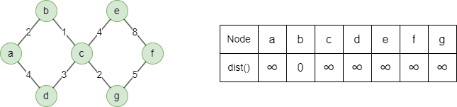
Below is an example of finding the weighted shortest path from source node b to target node g in an undirected graph:
1. Create a priority queue to store nodes and their corresponding distances from the source node. Initialize the distance of the source node as 0 and the distances of other nodes as infinity. All nodes are marked as unvisited.
2. Visit node u with the minimum distance from the queue, mark it as visited, and update the distance of each of its unvisited neighbors v as dist(v) = min(dist(u) + w(u,v), dist(v)), where w(u,v) is the weight of edge (u,v).
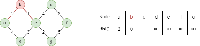
b: dist(a) = min(0+2,∞) = 2, dist(c) = min(0+1,∞) = 1NOTEOnce a node is marked as visited, its distance from the source node will no longer change throughout the remainder of the algorithm.
3. Repeat step 2 until the target node is visited.
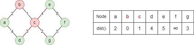
c: dist(d) = min(1+3, ∞) = 4, dist(e) = min(1+4, ∞) = 5, dist(g) = min(1+2, ∞) = 3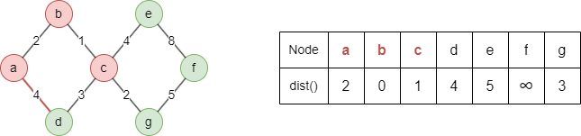
a: dist(d) = min(2+4, 4) = 4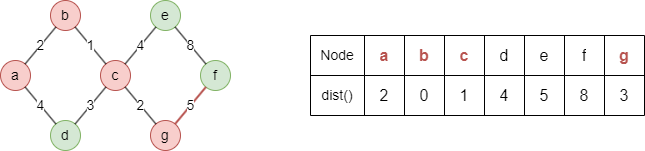
g: dist(f) = min(3+5, ∞) = 8The algorithm ends here as the target node g is visited. The shortest distance from node b to node g is 3.
Considerations
- Dijkstra doesn't work with negative weights — it assumes once a node is visited, its distance is final. A negative-weight edge could later provide a shorter path, violating this assumption.
Example Graph

GQLINSERT (A:default {_id: "A"}), (B:default {_id: "B"}),
       (C:default {_id: "C"}), (D:default {_id: "D"}),
       (E:default {_id: "E"}), (F:default {_id: "F"}),
       (G:default {_id: "G"}),
       (A)-[:default {value: 2}]->(B), (A)-[:default {value: 4}]->(F),
       (B)-[:default {value: 3}]->(C), (B)-[:default {value: 3}]->(D),
       (B)-[:default {value: 6}]->(F), (D)-[:default {value: 2}]->(E),
       (D)-[:default {value: 2}]->(F), (E)-[:default {value: 3}]->(G),
       (F)-[:default {value: 1}]->(E)
Parameters
| Name | Type | Default | Description |
|---|---|---|---|
source | STRING | / | Required. Source node _id. |
target | STRING | / | Required. Target node _id. |
weight | STRING | / | Numeric edge property to use as weight. If unset, all edges have unit weight. |
direction | STRING | out | Edge direction: in, out, or both. |
Run Mode
Returns:
| Column | Type | Description |
|---|---|---|
nodeId | STRING | Node identifier (_id) in the path |
cost | FLOAT | Total cost to reach this node from source |
index | INT | Position in the path (0 = source) |
path | STRING | Full path as string |
GQLCALL algo.shortestpath({
  source: "A",
  target: "G",
  weight: "value"
}) YIELD nodeId, cost, index, path
Result:
| nodeId | cost | index | path |
|---|---|---|---|
| A | 0 | 0 | A -> F -> E -> G |
| F | 4 | 1 | A -> F -> E -> G |
| E | 5 | 2 | A -> F -> E -> G |
| G | 8 | 3 | A -> F -> E -> G |
Stream Mode
Returns the same columns as run mode, streamed for memory efficiency.
GQLCALL algo.shortestpath.stream({
  source: "A",
  target: "G",
  weight: "value"
}) YIELD nodeId, cost
RETURN nodeId, cost
Result:
| nodeId | cost |
|---|---|
| A | 0 |
| F | 4 |
| E | 5 |
| G | 8 |
Stats Mode
Returns:
| Column | Type | Description |
|---|---|---|
nodeCount | INT | Number of nodes in the shortest path |
totalCost | FLOAT | Total cost of the shortest path |
GQLCALL algo.shortestpath.stats({
  source: "A",
  target: "G"
}) YIELD nodeCount, totalCost
Result:
| nodeCount | totalCost |
|---|---|
| 4 | 3 |