k-Edge Connected Components
Overview
The k-Edge Connected Components algorithm finds groups of nodes that have strong interconnections based on their edges. By considering the connectivity of edges rather than just the nodes themselves, the algorithm can reveal clusters within the graph where nodes are tightly linked to each other. This information can be valuable for social network analysis, web graph analysis, biological network analysis, and more.
Related material of the algorithm:
- T. Wang, Y. Zhang, F.Y.L. Chin, H. Ting, Y.H. Tsin, S. Poon, A Simple Algorithm for Finding All k-Edge-Connected Components (2015)
Concepts
Edge Connectivity
The edge connectivity of a graph is a measure that quantifies the minimum number of edges that need to be removed in order to disconnect the graph or reduce its connectivity. Given a graph G = (V, E), G is k-edge connected if it remains connected after the removal of any k-1 or fewer edges from G.
The edge connectivity can also be interpreted as the maximum number of edge-disjoint paths between any two nodes in the graph. If the edge connectivity of a graph is k, it means that there are k edge-disjoint paths between any pair of nodes in the graph.
Below shows a 3-edge connected graph and the edge-disjoint paths between each node pair.
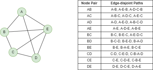
NOTEEdge-disjoint paths are paths that do not have any edge in common.
k-Edge Connected Components
Instead of determining whether the entire graph G is k-edge connected, the algorithm finds the maximal subsets of nodes Vi ⊆ V, where the subgraphs induced by Vi are k-edge connected.
For example, in social networks, finding a group of people who are strongly connected is more important than computing the connectivity of the entire social network.
Considerations
- The algorithm is exact for
k = 2. Fork ≥ 3, it uses a conservative approximation via iterative bridge removal and degree peeling. - The algorithm treats all edges as undirected.
Example Graph
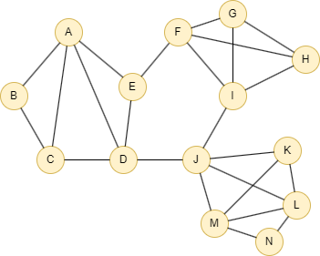
GQLINSERT (A:default {_id: "A"}), (B:default {_id: "B"}),
       (C:default {_id: "C"}), (D:default {_id: "D"}),
       (E:default {_id: "E"}), (F:default {_id: "F"}),
       (G:default {_id: "G"}), (H:default {_id: "H"}),
       (I:default {_id: "I"}), (J:default {_id: "J"}),
       (K:default {_id: "K"}), (L:default {_id: "L"}),
       (M:default {_id: "M"}), (N:default {_id: "N"}),
       (A)-[:default]->(B), (B)-[:default]->(C),
       (A)-[:default]->(C), (A)-[:default]->(D),
       (A)-[:default]->(E), (C)-[:default]->(D),
       (E)-[:default]->(D), (E)-[:default]->(F),
       (D)-[:default]->(J), (F)-[:default]->(G),
       (F)-[:default]->(I), (G)-[:default]->(H),
       (F)-[:default]->(H), (G)-[:default]->(I),
       (H)-[:default]->(I), (I)-[:default]->(J),
       (J)-[:default]->(K), (J)-[:default]->(M),
       (K)-[:default]->(L), (J)-[:default]->(L),
       (M)-[:default]->(K), (M)-[:default]->(L),
       (M)-[:default]->(N), (N)-[:default]->(L)
Parameters
| Name | Type | Default | Description |
|---|---|---|---|
k | INT | 2 | Edge connectivity requirement (k ≥ 2). |
Run Mode
Returns:
| Column | Type | Description |
|---|---|---|
nodeId | STRING | Node identifier (_id) |
componentId | INT | Component identifier |
GQLCALL algo.kedgeconnected({
  k: 3
}) YIELD nodeId, componentId
Result:
| nodeId | componentId |
|---|---|
| E | 0 |
| D | 1 |
| G | 2 |
| F | 2 |
| A | 3 |
| C | 4 |
| B | 5 |
| M | 6 |
| L | 6 |
| N | 7 |
| I | 2 |
| H | 2 |
| K | 6 |
| J | 6 |
Stream Mode
Returns the same columns as run mode, streamed for memory efficiency.
GQLCALL algo.kedgeconnected.stream({
  k: 3
}) YIELD nodeId, componentId
RETURN componentId, COLLECT(nodeId) AS members
GROUP BY componentId
Result:
| componentId | members |
|---|---|
| 0 | ["E"] |
| 1 | ["D"] |
| 2 | ["G", "F", "I", "H"] |
| 3 | ["A"] |
| 4 | ["C"] |
| 5 | ["B"] |
| 6 | ["M", "L", "K", "J"] |
| 7 | ["N"] |
Stats Mode
Returns:
| Column | Type | Description |
|---|---|---|
nodeCount | INT | Total number of nodes |
componentCount | INT | Number of k-edge-connected components |
largestComponentSize | INT | Size of the largest component |
smallestComponentSize | INT | Size of the smallest component |
GQLCALL algo.kedgeconnected.stats({
  k: 3
}) YIELD nodeCount, componentCount, largestComponentSize, smallestComponentSize
Result:
| nodeCount | componentCount | largestComponentSize | smallestComponentSize |
|---|---|---|---|
| 14 | 8 | 4 | 1 |
Write Mode
Computes results and writes them back to node properties. The write configuration is passed as a second argument map.
Write parameters:
| Name | Type | Description |
|---|---|---|
db.property | STRING or MAP | Node property to write results to. String: writes the componentId column in results to a property. Map: explicit column-to-property mapping (e.g., {componentId: 'kecc_id'}). |
Writable columns:
| Column | Type | Description |
|---|---|---|
componentId | INT | Component identifier |
Returns:
| Column | Type | Description |
|---|---|---|
task_id | STRING | Task identifier for tracking via SHOW TASKS |
nodesWritten | INT | Number of nodes with properties written |
computeTimeMs | INT | Time spent computing the algorithm (milliseconds) |
writeTimeMs | INT | Time spent writing properties to storage (milliseconds) |
GQLCALL algo.kedgeconnected.write({k: 3}, {
  db: {
    property: "kecc_id"
  }
}) YIELD task_id, nodesWritten, computeTimeMs, writeTimeMs