Eigenvector Centrality
Overview
Eigenvector centrality quantifies a node's influence within a graph. A node's importance is determined by its neighbors—it is both influenced by them and exerts influence on them. However, not all connections are equal; a node's centrality increases if it is connected to other highly influential nodes.
Eigenvector centrality scores range from 0 to 1; nodes with higher scores are more influential in the network.
Concepts
Eigenvector Centrality
The influence of a node is computed in a recursive way. Consider the graph below, and assume that nodes receive influence through incoming edges. In the adjacency matrix A, element Aij reflects the number of incoming edges of node i. Initially, each node is randomly assigned a centrality value — all set to 1 as an example —represented by the vector c(0).
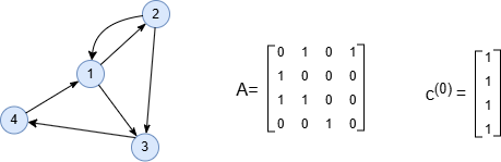
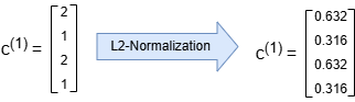
In each round of influence propagation, a node's centrality is updated as the sum of centralities of all its incoming neighbors. In the first round, this operation is equivalent to multiplying the vector c(0) by the matrix A, i.e., c(1) = Ac(0). Afterward, the L2-normalization is applied to rescale the vector c(1):
After k rounds, c(k) is computed by c(k) = Ac(k-1). As k grows, c(k) stabilizes. In this example, stabilization is reached after approximately 20 rounds. The elements in c(k) represent the centrality of the corresponding nodes.

The algorithm continues until the sum of changes of all elements in c(k) converges to within some tolerance, or the maximum iteration rounds is met.
Eigenvalue and Eigenvector
Given that A is an n x n square matrix, λ is a constant, and x is a non-zero n x 1 vector. If the equation Ax = λx is true, then λ is called the eigenvalue of A, and x is the eigenvector of A that corresponds to λ.
The above adjacency matrix A has four eigenvalues λ1, λ2, λ3 and λ4 that correspond to eigenvectors x1, x2, x3 and x4, respectively. x1 is the eigenvector of the eigenvalue λ1 which has the largtest absolute value. λ1 is the dominant eigenvalue, and x1 the dominant eigenvector.

In fact, as k grows, c(k) always converges to x1, regardless of how c(0) is initialized. This phenomenon is explained by the Perron–Frobenius theorem. Therefore, computing the eigenvector centrality of nodes in a graph is equivalent to finding the dominant eigenvector of the adjacency matrix A.
Considerations
- A self-loop counts as one in-link and one out-link.
Example Graph
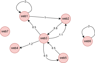
GQLINSERT (web1:web {_id: "web1"}), (web2:web {_id: "web2"}),
       (web3:web {_id: "web3"}), (web4:web {_id: "web4"}),
       (web5:web {_id: "web5"}), (web6:web {_id: "web6"}),
       (web7:web {_id: "web7"}),
       (web1)-[:link {value: 2}]->(web1), (web1)-[:link {value: 1}]->(web2),
       (web2)-[:link {value: 0.8}]->(web3), (web3)-[:link {value: 0.5}]->(web1),
       (web3)-[:link {value: 1.1}]->(web2), (web3)-[:link {value: 1.2}]->(web4),
       (web3)-[:link {value: 0.5}]->(web5), (web5)-[:link {value: 0.5}]->(web3),
       (web6)-[:link {value: 2}]->(web6)
Parameters
| Name | Type | Default | Description |
|---|---|---|---|
ids | LIST | / | _ids of nodes to compute (empty = all nodes). |
direction | STRING | both | Edge direction: in, out, or both. |
maxIterations | INT | 100 | Maximum number of iterations. |
tolerance | FLOAT | 0.000001 | Convergence tolerance. The algorithm terminates when score changes between iterations are less than this value. |
weight | STRING or LIST | / | Numeric edge property for weighted adjacency. |
limit | INT | -1 | Limits the number of results returned (-1 = all). |
order | STRING | / | Sorts the results by score: asc or desc. |
Run Mode
Returns:
| Column | Type | Description |
|---|---|---|
nodeId | STRING | Node identifier (_id) |
score | FLOAT | Eigenvector centrality score |
rank | INT | Rank position (1 = highest eigenvector centrality) |
Eigenvector centrality for all nodes:
GQLCALL algo.eigenvector({
  maxIterations: 50,
  tolerance: 0.000001,
  direction: "in",
  order: "desc"
}) YIELD nodeId, score, rank
Result:
| nodeId | score | rank |
|---|---|---|
| web1 | 0.5736120501246498 | 1 |
| web2 | 0.5736120501246498 | 2 |
| web3 | 0.4600016017850023 | 3 |
| web5 | 0.25528117660613436 | 4 |
| web4 | 0.25528117660613436 | 5 |
| web6 | 1.7088326722892042e-9 | 6 |
| web7 | 0 | 7 |
Stream Mode
Returns the same columns as run mode, streamed for memory efficiency.
GQLCALL algo.eigenvector.stream({
  maxIterations: 300,
  tolerance: 0.000001,
  weight: ["value"],
  direction: "in",
  order: "desc"
}) YIELD nodeId, score
RETURN nodeId, score
Result:
| nodeId | score |
|---|---|
| web1 | 0.8354748144328726 |
| web2 | 0.4975228759458507 |
| web3 | 0.19890390105629813 |
| web4 | 0.11263830879446735 |
| web5 | 0.046932628664361396 |
| web6 | 0.000016189148967104193 |
| web7 | 0 |
Stats Mode
Returns:
| Column | Type | Description |
|---|---|---|
nodeCount | INT | Total number of nodes |
minScore | FLOAT | Minimum eigenvector centrality score |
maxScore | FLOAT | Maximum eigenvector centrality score |
avgScore | FLOAT | Average eigenvector centrality score |
GQLCALL algo.eigenvector.stats() YIELD nodeCount, minScore, maxScore, avgScore
Result:
| nodeCount | minScore | maxScore | avgScore |
|---|---|---|---|
| 7 | 0 | 0.6195366525240715 | 0.2951366032678612 |
Write Mode
Computes results and writes them back to node properties. The write configuration is passed as a second argument map.
Write parameters:
| Name | Type | Description |
|---|---|---|
db.property | STRING or MAP | Node property to write results to. String: writes the score column in results to a property. Map: explicit column-to-property mapping (e.g., {score: 'ec_score', rank: 'ec_rank'}). |
Writable columns:
| Column | Type | Description |
|---|---|---|
score | FLOAT | Eigenvector centrality score |
rank | INT | Rank position |
Returns:
| Column | Type | Description |
|---|---|---|
task_id | STRING | Task identifier for tracking via SHOW TASKS |
nodesWritten | INT | Number of nodes with properties written |
computeTimeMs | INT | Time spent computing the algorithm (milliseconds) |
writeTimeMs | INT | Time spent writing properties to storage (milliseconds) |
GQLCALL algo.eigenvector.write({}, {
  db: {
    property: "ec_score"
  }
}) YIELD task_id, nodesWritten, computeTimeMs, writeTimeMs