LINE
Overview
LINE (Large-scale Information Network Embedding) is a network embedding model that preserves the local or global network structures. LINE is able to scale to very large, arbitrary types of networks, it was originally proposed in 2015:
- J. Tang, M. Qu, M. Wang, M. Zhang, J. Yan, Q. Zhu, LINE: Large-scale Information Network Embedding (2015)
Concepts
First-order Proximity and Second-order Proximity
First-order proximity in a network shows the local proximity between two nodes, and it is contingent upon connectivity. A link between two nodes—or a stronger (positive) link weight—indicates higher first-order proximity. If no link exists between them, their first-order proximity is considered 0.
On the other hand, second-order proximity measures the similarity between the neighborhood structures of two nodes, based on shared neighbors. If two nodes have no common neighbors, their second-order proximity is 0.
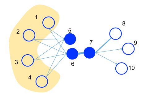
In this graph, the edge thickness signifies its weight:
- A substantial weight on the edge between nodes 6 and 7 indicates a strong first-order proximity, meaning they should have similar representations in the embedding space.
- Although nodes 5 and 6 are not directly connected, their considerable common neighbors create a significant second-order proximity. As a result, they are also expected to be represented close to each other in the embedding space.
LINE Model
The LINE model is designed to embed nodes in graph G = (V,E) into low-dimensional vectors, while preserving either the first-order or second-order proximity between nodes.
First-order Proximity
To capture the first-order proximity, LINE defines the joint probability for each edge (i,j) ∈ E connecting nodes vi and vj as:
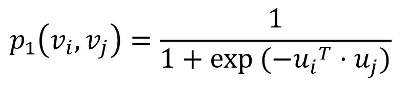
where ui is the vector representation of node vi. p1 ranges from 0 to 1: the closer the vectors (i.e., the higher their dot product), the higher the joint probability.
Empirically, the joint probability between node vi and vj is defined as:
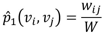
where wij denotes the edge weight between two nodes, W is the sum of all edge weights in the graph.
The KL-divergence is adopted to measure the difference between p1 (model's prediction) and p̂1 (ground truth):
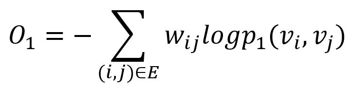
This serves as the objective function that needs to be minimized during training when preserving the first-order proximity.
Second-order Proximity
To model the second-order proximity, LINE defines two roles for each node: one as the node itself, another as "context" for other nodes. For each edge (i,j) ∈ E, LINE defines the probability of "context" vj be observed by node vi as:
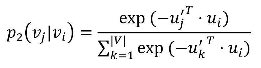
where u'j is the representation of node vj when it is regarded as the "context". Importantly, the denominator involves the whole "context" in the graph.
The corresponding empirical probability is defined as:
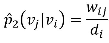
where wij is weight of edge (i,j), di is the weighted degree of node vi.
Similarly, the KL-divergence is adopted to measure the difference between p2 (model's prediction) and p̂2 (ground truth):
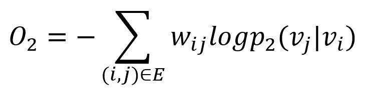
This serves as the objective function that needs to be minimized during training when preserving the second-order proximity.
Model Optimization
Negative Sampling
To improve computation efficiency, LINE uses negative sampling, drawing multiple negative edges from a noise distribution for each edge (i,j). The two objective functions are adjusted as:
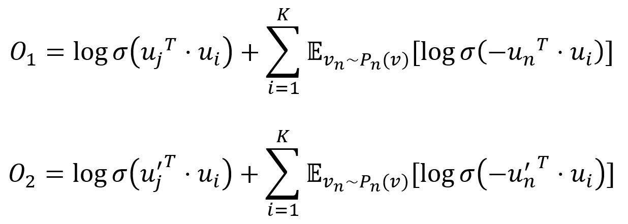
where σ is the sigmoid function, K is the number of negative edges drawn from the noise distribution Pn(v) ∝ dv3/4, dv is the weighted degree of node v.
Edge-Sampling
Since edge weights are included in both objective functions, they are also applied to the gradients during optimization. This can cause gradient explosion and degrade model performance. To address this, LINE samples edges with probabilities proportional to their weights and treats the sampled edges as binary during model updates.
Considerations
- The LINE algorithm treats all edges as undirected, ignoring their original direction.
Example Graph
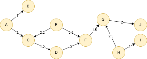
GQLINSERT (A:default {_id: "A"}), (B:default {_id: "B"}),
       (C:default {_id: "C"}), (D:default {_id: "D"}),
       (E:default {_id: "E"}), (F:default {_id: "F"}),
       (G:default {_id: "G"}), (H:default {_id: "H"}),
       (I:default {_id: "I"}), (J:default {_id: "J"}),
       (K:default {_id: "K"}),
       (A)-[:default]->(B), (A)-[:default]->(C),
       (C)-[:default]->(D), (D)-[:default]->(C),
       (D)-[:default]->(F), (E)-[:default]->(C),
       (E)-[:default]->(F), (F)-[:default]->(G),
       (G)-[:default]->(J), (H)-[:default]->(G),
       (H)-[:default]->(I), (I)-[:default]->(I),
       (J)-[:default]->(G)
Parameters
| Name | Type | Default | Description |
|---|---|---|---|
dimensions | INT | 128 | Embedding dimensionality. |
order | INT | 2 | Proximity order: 1 for first-order, 2 for second-order, 3 for both (concatenated). |
negSamples | INT | 5 | Number of negative samples per edge. |
iterations | INT | 5 | Number of SGD training iterations. |
learningRate | FLOAT | 0.025 | Initial learning rate for SGD. |
Run Mode
Returns:
| Column | Type | Description |
|---|---|---|
nodeId | STRING | Node identifier (_id) |
embedding | LIST | Embedding vector as list of floats |
GQLCALL algo.line({
  dimensions: 4,
  order: 1,
  iterations: 10
}) YIELD nodeId, embedding
Stream Mode
Returns the same columns as run mode, streamed for memory efficiency.
GQLCALL algo.line.stream({
  dimensions: 4,
  order: 2
}) YIELD nodeId, embedding
RETURN nodeId, embedding
Stats Mode
Returns:
| Column | Type | Description |
|---|---|---|
nodeCount | INT | Total number of nodes processed |
dimensions | INT | Embedding dimensionality |
GQLCALL algo.line.stats({
  dimensions: 4
}) YIELD nodeCount, dimensions
Write Mode
Computes results and writes them back to node properties. The write configuration is passed as a second argument map.
Write parameters:
| Name | Type | Description |
|---|---|---|
db.property | STRING or MAP | Node property to write results to. |
Writable columns:
| Column | Type | Description |
|---|---|---|
embedding | LIST | Embedding vector |
Returns:
| Column | Type | Description |
|---|---|---|
task_id | STRING | Task identifier for tracking via SHOW TASKS |
nodesWritten | INT | Number of nodes with properties written |
computeTimeMs | INT | Time spent computing the algorithm (milliseconds) |
writeTimeMs | INT | Time spent writing properties to storage (milliseconds) |
GQLCALL algo.line.write({dimensions: 4, order: 1}, {
  db: {
    property: "embedding"
  }
}) YIELD task_id, nodesWritten, computeTimeMs, writeTimeMs