k-Core
Overview
The k-Core algorithm performs k-core decomposition, computing the coreness of each node — the maximum k for which the node belongs to a k-core subgraph. It is commonly employed to identify tightly connected groups in a graph for further analysis. Common applications include financial risk control, social network analysis, and biological studies. The algorithm runs in linear time, making it efficient for large graphs.
The widely accepted concept of k-core was first introduced by Seidman:
- S.B. Seidman, Network Structure And Minimum Degree. Soc Netw 5:269-287 (1983)
Concepts
k-Core
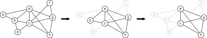
The k-core of a graph is the largest subgraph where every node has at least degree k. It is computed through iterative pruning: nodes with degree less than k are successively removed until all remaining nodes have degrees ≥ k.
Below is the pruning process to get the 3-core of the graph. In the first round, nodes {a, d, f} with degree less than 3 are removed, which then affects the removal of node b in the second round. After the second round, all remaining nodes have a degree of at least 3. Therefore, the pruning process ends, and the 3-core of this graph is induced by nodes {c, e, g, h}.
Coreness
The coreness of a node is the maximum k for which the node belongs to a k-core. For example, if a node is in the 3-core but not in the 4-core, its coreness is 3. This algorithm computes the coreness for every node in the graph.
The algorithm computes coreness across all connected components independently.
Considerations
- The algorithm ignores self-loops when calculating degree.
- The algorithm treats all edges as undirected.
Example Graph
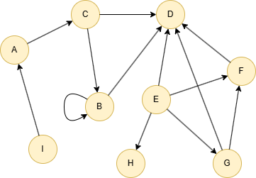
GQLINSERT (A:default {_id: "A"}), (B:default {_id: "B"}),
       (C:default {_id: "C"}), (D:default {_id: "D"}),
       (E:default {_id: "E"}), (F:default {_id: "F"}),
       (G:default {_id: "G"}), (H:default {_id: "H"}),
       (I:default {_id: "I"}),
       (A)-[:default]->(C), (B)-[:default]->(B),
       (B)-[:default]->(D), (C)-[:default]->(B),
       (C)-[:default]->(D), (E)-[:default]->(D),
       (E)-[:default]->(F), (E)-[:default]->(G),
       (E)-[:default]->(H), (F)-[:default]->(D),
       (G)-[:default]->(D), (G)-[:default]->(F),
       (I)-[:default]->(A)
Parameters
| Name | Type | Default | Description |
|---|---|---|---|
limit | INT | -1 | Limits the number of results returned (-1 = all). |
order | STRING | / | Sorts the results by coreness: asc or desc. |
Run Mode
Returns:
| Column | Type | Description |
|---|---|---|
nodeId | STRING | Node identifier (_id) |
coreness | INT | The maximum k-core the node belongs to |
degree | INT | The node's degree |
GQLCALL algo.kcore() YIELD nodeId, coreness, degree
Result:
| nodeId | coreness | degree |
|---|---|---|
| E | 3 | 4 |
| D | 3 | 5 |
| G | 3 | 3 |
| F | 3 | 3 |
| A | 1 | 2 |
| C | 2 | 3 |
| B | 2 | 2 |
| I | 1 | 1 |
| H | 1 | 1 |
Stream Mode
Returns the same columns as run mode, streamed for memory efficiency.
GQLCALL algo.kcore.stream() YIELD nodeId, coreness
FILTER coreness >= 3
RETURN nodeId, coreness
Result:
| nodeId | coreness |
|---|---|
| E | 3 |
| D | 3 |
| G | 3 |
| F | 3 |
Stats Mode
Returns:
| Column | Type | Description |
|---|---|---|
nodeCount | INT | Total number of nodes |
maxCoreness | INT | Maximum coreness value |
avgCoreness | FLOAT | Average coreness value |
GQLCALL algo.kcore.stats() YIELD nodeCount, maxCoreness, avgCoreness
Result:
| nodeCount | maxCoreness | avgCoreness |
|---|---|---|
| 9 | 3 | 2.111111111111111 |
Write Mode
Computes results and writes them back to node properties. The write configuration is passed as a second argument map.
Write parameters:
| Name | Type | Description |
|---|---|---|
db.property | STRING or MAP | Node property to write results to. String: writes the coreness column in results to a property. Map: explicit column-to-property mapping (e.g., {coreness: 'core', degree: 'deg'}). |
Writable columns:
| Column | Type | Description |
|---|---|---|
coreness | INT | Coreness value |
degree | INT | Node degree |
Returns:
| Column | Type | Description |
|---|---|---|
task_id | STRING | Task identifier for tracking via SHOW TASKS |
nodesWritten | INT | Number of nodes with properties written |
computeTimeMs | INT | Time spent computing the algorithm (milliseconds) |
writeTimeMs | INT | Time spent writing properties to storage (milliseconds) |
GQLCALL algo.kcore.write({}, {
  db: {
    property: "coreness"
  }
}) YIELD task_id, nodesWritten, computeTimeMs, writeTimeMs