Bipartite Graph
Overview
The Bipartite algorithm determines whether a given graph is a bipartite graph and assigns each node to one of two partitions. The algorithm uses BFS 2-coloring to identify and leverage the structure of bipartite graphs, enabling efficient resource allocation, task assignment, and group optimization.
Concepts
Bipartite Graph
A bipartite graph, also known as a bigraph, is a graph in which the nodes can be divided into two disjoint sets such that every edge connects a node from one set to a node in the other. In other words, no edge connects nodes within the same set.
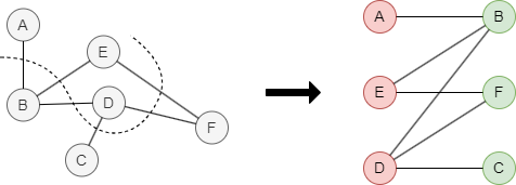
This example graph is bipartite. The nodes can be partitioned into sets V1 = {A, D, E} and V2 = {B, C, F}.
Coloring Method
To determine if a graph is bipartite, one common approach is to perform a graph traversal and assign each visited node to one of two different sets. This process is often referred to as "coloring" the nodes. During traversal, if an edge is found that connects two nodes within the same set, the graph is not bipartite. Conversely, if all edges connect nodes from different sets, the graph is bipartite.
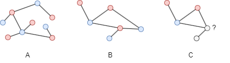
In this example, both graph A and graph B are bipartite. Graph C is not bipartite as it contains an odd cycle. An odd cycle is a cycle that has an odd number of nodes. Bipartite graphs cannot contain odd cycles, as it is impossible to color all nodes in an odd cycle using only two colors while satisfying the bipartite condition.
Considerations
- A self-loop connects a node to itself, meaning both endpoints are the same node. Therefore, any graph containing a self-loop is not bipartite.
- The algorithm treats all edges as undirected.
Example Graph
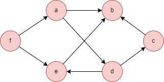
GQLINSERT (a:default {_id: "a"}), (b:default {_id: "b"}),
       (c:default {_id: "c"}), (d:default {_id: "d"}),
       (e:default {_id: "e"}), (f:default {_id: "f"}),
       (a)-[:default]->(b), (a)-[:default]->(d),
       (c)-[:default]->(b), (d)-[:default]->(c),
       (d)-[:default]->(e), (e)-[:default]->(b),
       (f)-[:default]->(a), (f)-[:default]->(e)
Run Mode
Returns:
| Column | Type | Description |
|---|---|---|
nodeId | STRING | Node identifier (_id) |
partition | INT | Partition assignment (0 or 1; -1 if the component is not bipartite) |
isBipartite | INT | 1 if the component containing this node is bipartite, 0 otherwise |
GQLCALL algo.bipartite() YIELD nodeId, partition, isBipartite
Result:
| nodeId | partition | isBipartite |
|---|---|---|
| e | 0 | 1 |
| d | 1 | 1 |
| f | 1 | 1 |
| a | 0 | 1 |
| c | 0 | 1 |
| b | 1 | 1 |
Stream Mode
Returns the same columns as run mode, streamed for memory efficiency.
GQLCALL algo.bipartite.stream() YIELD nodeId, partition
RETURN partition, COLLECT(nodeId) AS nodes
GROUP BY partition
Result:
| partition | nodes |
|---|---|
| 0 | ["e", "a", "c"] |
| 1 | ["d", "f", "b"] |
Stats Mode
Returns:
| Column | Type | Description |
|---|---|---|
nodeCount | INT | Total number of nodes |
isBipartite | INT | 1 if the entire graph is bipartite, 0 otherwise |
partition0Size | INT | Number of nodes in partition 0 |
partition1Size | INT | Number of nodes in partition 1 |
componentCount | INT | Number of connected components |
GQLCALL algo.bipartite.stats() YIELD nodeCount, isBipartite, partition0Size, partition1Size, componentCount
Result:
| nodeCount | isBipartite | partition0Size | partition1Size | componentCount |
|---|---|---|---|---|
| 6 | 1 | 3 | 3 | 1 |