By Ricky Sun and Jason Zhang

Admittedly, we are now living in an era of big data. The rapid evolvement of the Internet and mobile internet has greatly boosted the rate of data generated, there are billions of devices, some even predicting the arrival of trillions of sensory devices within this decade, generating a gigantic volume of data.

Database was created to tackle this ever-growing data challenge. There were other concepts and solutions like data mart, data warehouse, and data lake created to cater to the needs of data storage, transformation, intelligent analysis, reporting, and many other things. But what makes database essentially indispensable are mainly two promises with regards to the ability to process all aforementioned tasks:

• Performance
• Query Language

In the world of modern business, performance has always been a first-class citizen. A database can be called database manifests due to its processing power against data with small, and usually minimal and business-sense-making, latencies. This is in contrast with many BI-era data warehouse solutions or Hadoop-school solutions, which may be highly distributed and scalable but with performances that are quite worrisome. And this is exactly why we are seeing the dying of Hadoop (or replacement with Spark and other newer architectures) in recent years.

The trend of moving from Big Data to Fast Data is to ensure that given the growing data volume, the underpinning database frameworks can handle it without sacrificing performance. The below diagram illustrates the evolvement of database-centric data processing technologies. In short, we would like to summarize the trend as Data →  Big Data → Fast Data → Deep Data. Let’s not worry about the new concepts (fast or deep) here, we’ll get to them momentarily.

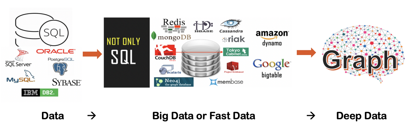
Diagram-0: The Evolution of Data to Big Data to Fast Data to Deep Data

Query language is one of the best things ever invented since computer programming language is invented. Ideally, we want our computer programs to have the ability to sift through data with human-grade intelligence, but this goal of 'strong AI' has never been fully achieved. As a fallback solution, smart programmers and computer linguists created artificial languages to help translate human orders into computer instructions, and these artificial languages are the query languages that are supported by databases to facilitate data processing.

Before we dive into the well-known SQL world, allow us to elaborate a little bit about query languages used by certain NoSQL or non-RDBMS data stores, which can be loosely taken as databases.

First, let’s examine KV Store, which is short for Key-Value Database, the popular implementations including Berkeley DB, Level DB, and etc. Technically speaking, KV store does NOT utilize a specific query language. This is mainly due to their rather straightforward operations, which make a simple API suffice. A typical KV store’s API supports 3 operations:

• Insert
• Get
• Delete

You may argue that Cassandra does have CQL (Cassandra Query Language). No problem with that. Cassandra is a wide-column store, which can be seen as a two-dimensional KV-store, and for the complexity of data operations in and out of Cassandra’s highly distributed infrastructure, it does make sense to provide a layer of abstraction to ease the programmer’s load on memorizing all those burdensome API calling parameters. By the way, CQL uses similar concepts as regular SQL, such as tables, rows, and columns, we’ll get to SQL-specific discussions next.

One critique against Apache Cassandra, and NoSQL databases in general, is that JOIN queries are not supported in CQL as in SQL. Understandably, the critique is deeply rooted in a SQL way of thinking (but JOIN is a double-edged sword, it helps achieve one thing but brings about side effects like performance penalties…). There are actually ways to enable Cassandra with JOINs, for instance:

• ApacheSpark’s Spark SQL with Cassandra
• Cassandra with ODBC driver

However, these solutions are not without caveats, ODBC’s performance is problematic for large datasets or clusters, and Spark SQL atop Cassandra simply introduces yet another layer of complexities – which most programmers hate to deal with.

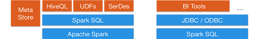
Diagram-1: Spark SQL for working with Apache Spark’s Structured Data

A few extra words about Apache Spark and Spark SQL. Spark was designed in light of the inefficiencies of Apache Hadoop, which borrows 2 key concepts from Google’s GFS and MapReduce and develops into Hadoop’s HDFS and MapReduce. Spark is 100x faster than Hadoop mainly due to its distributed shared-memory architecture design (To draw an analogy, by moving data to be stored and computed in memory, there is 100x performance gain over disk-based operations, period.). Spark SQL was invented to process Spark’s structured data by providing a SQL-compatible query language interface. It clearly is an advancement compared to Spark’s RDD API. As explained earlier, API can be less efficient when it’s getting overly complicated, and at that point, a query language is more desirable and practical (and flexible and powerful).   

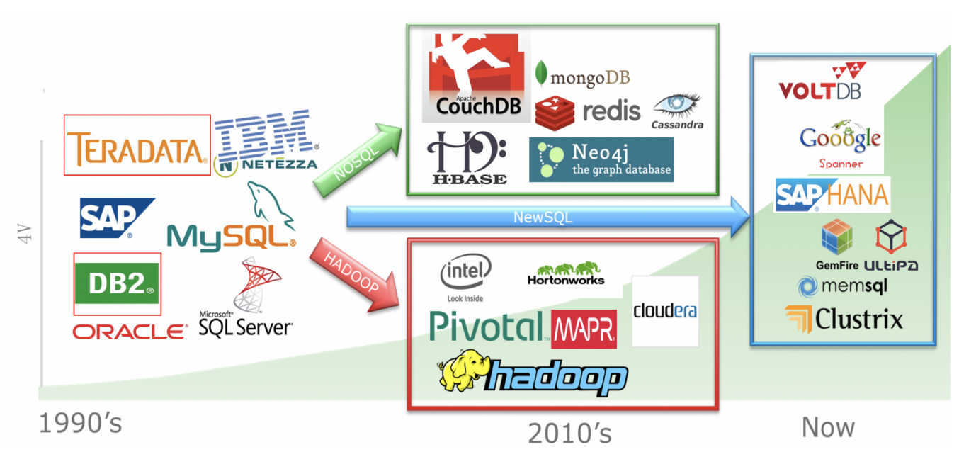
Diagram-2: The Evolvement of Database and Data-Processing Technologies

In Diagram-0, we have illustrated the industry-wide trend of moving from data to big-data then to fast data, so on and so forth. The underlying data-processing technologies are actually moving from relational databases to non-relational databases (NOSQLs and Hadoops), and to NewSQLs or graph database frameworks that are capable of big-data and fast data and even to the extent of deep data. This trend is captured in Diagram-2.

The evolution of database technologies in the past half-century has been cartooned as in Diagram-3 – evolving from 70-80s RDBMS with repetitive SQL enforcement in the 80-90s, and the rebels-n-breakthroughs by NoSQLs (Not-Only-SQLs) in the 00s-10s.

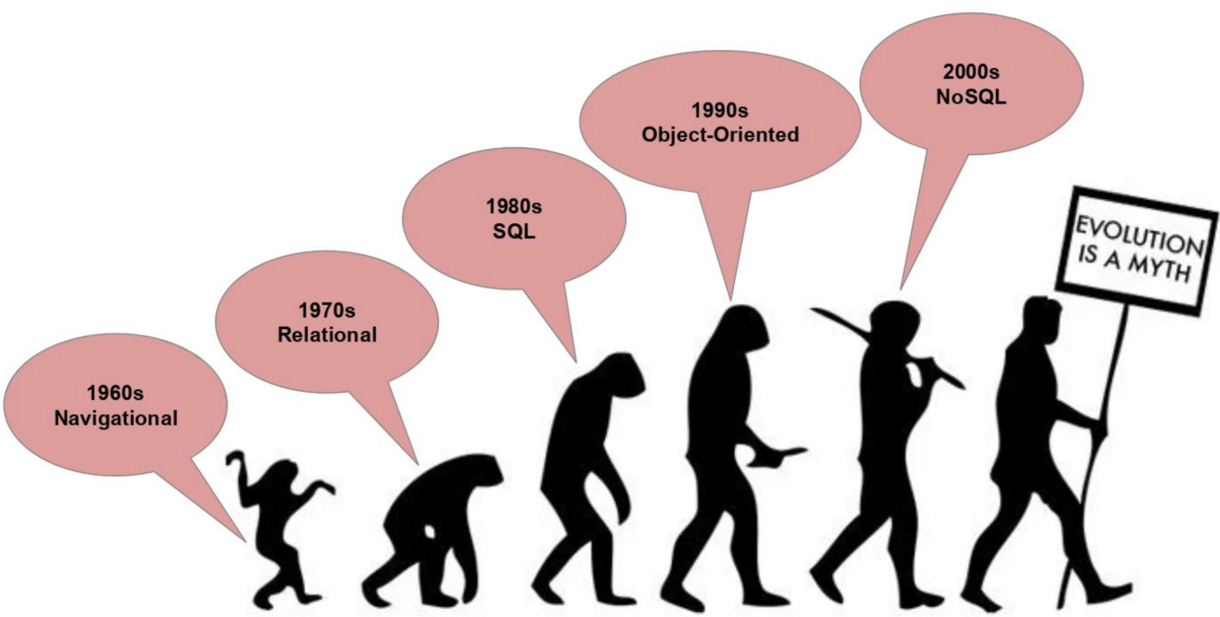
Diagram-3: Progressive View of Database Evolution

The evolvement of SQL gives rise to relational databases, and the rise of the Internet gives birth to NoSQL, mainly due to relational DBs' incapacity to cope with the need for speed and data-modeling flexibility.

There are basically 4 (or 5 if we may include Time Series) subtypes of NoSQL databases, each with its own characteristics:

• Key-Value: Performance and simplicity.
• Wide-Column: Volume and performance for data access.
• Document: Variety of data structures supported.
• Graph: Deep-data and fast-data.
• (optionally) Time Series:  Performance for time-stamped/IoT data.

In terms of query language (and/or API) complexity, some may argue that the advancement of data-processing capabilities has an evolutional path, the below diagram (Diagram-4) outlines how NoSQLs compare with SQL-centric RDBMS. And the path is from:

• The primitive key-value store type of API to Ordered Key-Value
• Ordered Key-value to Big-Table (Wide Column Store), to
• Document Database (i.e., MongoDB) with Full-Text Search (Search Engine), to
• Graph Database, and
• SQL-centric Relational Database.

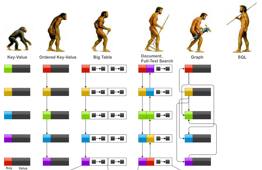
Diagram-4: A Reversed View of Database Query Language Evolution

In this view (per Diagram-4), SQL is considered the most modern and advanced way of processing data linguistically. Let’s take a slightly deeper look at SQL’s evolvement and this will help us better understand it, and if we include NoSQLs alongside, we’ll have a panoramic view.

SQL was invented about 50 years ago and has been revised for good many times, most notably the SQL-92 standard which added subquery functionality in the FROM clause, and CTE (Common Table Expression) feature which was added in SQL-99. These features infused great flexibility to relational databases; however, a major lacking persists – recursive data structures.

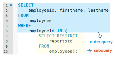
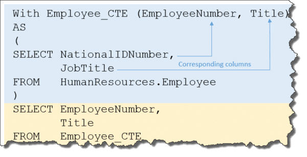
Diagram-5: Subquery per SQL-92 and CTE per SQL-99

While recursive data structures are basically directed graphs and relational databases were not designed with the concept of directed-graph in mind (therefore, ironically, relational databases are NOT relational at all), to achieve the goal of finding relations among data entities, RDBMS have to rely on table joins to retrieve data, this greatly slows down query performances (not to mention table-join also complicates SQL coding exponentially). The performance penalty associated with table joins are mainly due to the fundamental design philosophy of relational databases:

• Data Normalization
• Fixed/Predefined Schema

If we look at NoSQLs, the primary data-modeling design concept of most NoSQLs is data de-normalization. Data de-normalization is basically to trade time with space, meaning data may be stored in a multitude of copies, so that they can be accessed in a storage-in-close-proximity-to-compute way. This is in contrast to SQL’s just-one-copy all-data-normalized design, which may save some space, but tends to yield worse performance when dreadful SQL operations like table joins are necessary.

Pre-defined schema is another major difference between SQL and NoSQL, and this can be hard to conceptualize. One way to digest this is to think:

Schema First, Data Second vs. Data First, Schema Second

In a relational database, the administrator has to define table schema before loading any data into the database, and he/she can NOT change the schema on the fly. This rigidness may not be such a big issue if all your data are very steady and never-changing. But, let’s picture a scenario where schema can self-adjust or improvise to accommodate the inbound data, this gives maximum flexibility. For people with strong SQL background, this is hard to imagine, but let’s replace our fixed mindset with a growth mindset and see how to achieve 'Schemaless-ness'.

Over the past several decades, database programmers are trained to understand data model(s) first and foremost, be it a relational model which is table-specific, or an E-R model which is entity-specific. Understand that the data models have their clear benefits; however, this hinders development progress, slows things down, and makes a turn-key solution development cycle longer and potentially complicated.

By saying schema-free, we do NOT mean to explain the designs by document databases, or big-table-like wide-column tables, though they do bear similarities in terms of design philosophy to graph databases. We'll get to specific examples to help you understand what schema-free really means. 

In a graph database, there are 2 types of logically fundamental data types:

• Nodes (also called Vertices)
• Edges

A node may have its own ID and attributes (labels and tags and etc.); an edge is essentially comprised of 2 nodes with sequence and attributes. Other than these basic features, graph database does NOT require any pre-defined schema; to be frank, there is no need to define schemas. This simplistic concept is very similar to how we human beings store information – we do NOT pre-define table schemas, we improvise!

Now, let’s look at a real-world implementation. In Diagram-6, there are 2 highlighted attributes (name and type), which are considered basic, and every other attribute is dynamically created and removable.  

Diagram-6: A Graph Dataset, Nodes w/ Fixed and Dynamic Attributes

Note that both name and type attribute are STRING typed to accommodate broad spectrum data-type flexibility, so that node may have many data types and this does NOT dictate (define) how any two nodes are related, which leaves room for inter-node (edge) relationship to be flexible as well.

Of course, there are a lot of performance-related optimizations to the schema-free design illustrated in Diagram-6, such as tiering things up by loading certain data structures into memory for optimal computational throughput and vice versa (to offload to disk storage to save space).

Key-Value stores can be seen as pre-SQL and non-relational, while graph databases on the other hand are post-SQL and support truly recursive data structures. Lots of today’s NoSQL databases are supporting (or at least trying to support) SQL to be backward compatible; however, SQL is very much table-confined, and this is, in our humble opinion, counter-intuitive and in-efficient. By saying table-confined, we really mean it is two-dimensional thinking, and doing table join is like three-or-higher-dimensional thinking; but as the foundation in the data model is two-dimension based, the SQL framework is fundamentally restrictive!

Graph, on the other hand, is high-dimensional. Operations on graphs are also high dimensional, many of which are natively recursive. For instance, breadth-first-search (BFS) or depth-first-search (DFS). Moreover, graph can be backward compatible, which is to support SQL-like operations just as Spark, column, or KV stores do.

Let’s examine a few graph queries next, and please bear in mind and think about how SQL or other NoSQL would accomplish the same.

1. Starting from a node, find all its neighbors recursively up to K layers, and return the resulting dataset (sub-graph).  

To achieve this, in uQL — short for Ultipa Query Language, which is a high-performance parallel graph query language designed to offer a unison of maximum performance and intuitiveness, and with the flexibility to embed within Ultipa Manager (the graphical data manager) or Ultipa CLI (the command line interface) — a single line of code would suffice.

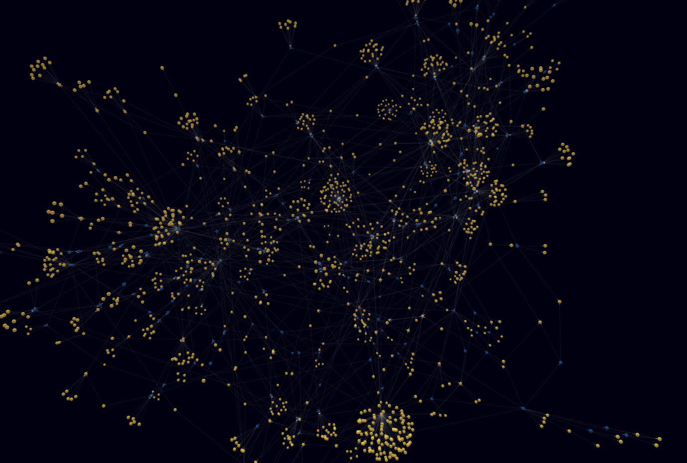
Diagram-7: A Holistic View of a Graph Dataset via node spread()

Here is the line of code:

nodeSpread().src(123).depth(6).spread_type("BFS").limit(4000);

The code itself is pretty much self-explainable, starting with the source code (ID=123), expanding in a BFS way for up to 6 hops, returning up to 4000 nodes (and edges, implicitly). In Diagram-7, the tiny red dot just below the center is the starting node. The resulting subgraph almost consists of the entire graph (a small one), therefore, we are calling it: a holistic view of the graph.

As a side note, the above diagram also shows how useful visualization can be. It intuitively shows the hot spots and entity relationships, without the burning need for an explicit E-R model.

2. Given a set of nodes, automatically forming a network (sub-graph) with a specific depth and number of paths.

This query takes little human cognitive load, but it would be extremely difficult to implement in a SQL setup (If you have doubt on this, try it yourself and let us know).

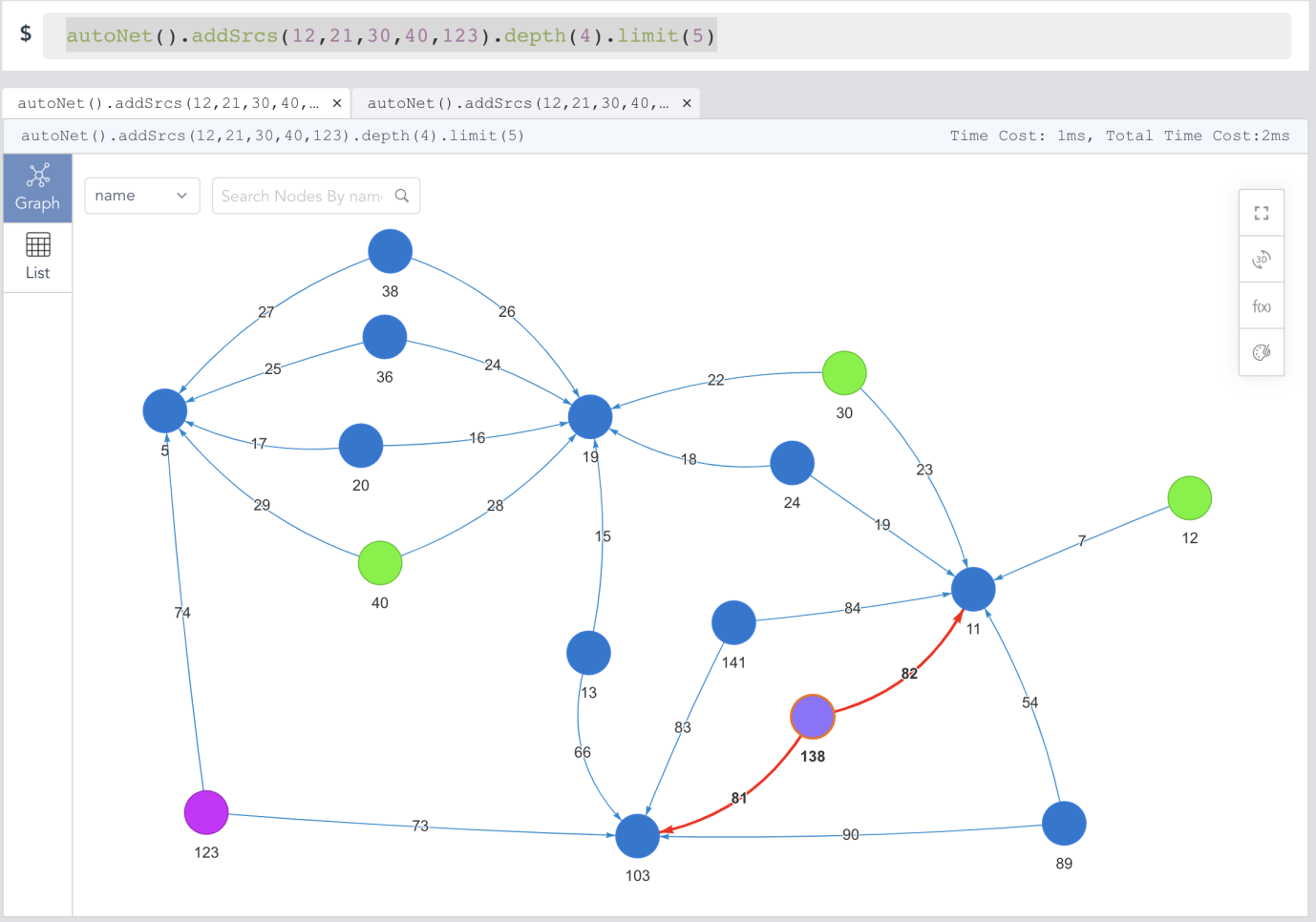
Diagram-8: Automatic Network or Subgraph Formation in Ultipa Graph

This is also a single line of code:

autoNet().addSrcs(12,21,30,40,123).depth(4).limit(5)

autoNet() is the function to call, the starting nodes are set with multiple vertices (as many as you desire), the path search depth between any 2 nodes is 4-hop, and the number of paths between any two nodes is limited to 5. Let’s straighten out this query mathematically so that we can have a better idea about how complex it is. The computational complexity is:

Paths to Return: C(5, 2) * 5 = (5 * 4 / 2) * 5 = 50 paths

Graph Calculations: 50 paths * (E/V)4 = 50 * 256 = 12800

Assuming E/V is the ratio of vertex-to-edge, let’s say this graph has E/V=4.

In real-world applications, law enforcement may query for crime rings by utilizing phone companies' call records, and by forming a big network, they can look into the characteristics of the resulting call networks for hints such as how close or distant any two suspects are and how they operate like gangs.

Traditionally, these operations are extremely time-consuming on any big-data frameworks and practically impossible with relational databases. The reason is computational complexity, assuming there are 1,000 suspects/gangsters/nodes to query against, there are (1,000 * 999) / 2 = 500K possible connections and unlimited possibilities if the query depth is 6-hop! Spark with GraphX may take days to calculate, but on Ultipa Graph, it's real-time or near real-time, possibly with a turnaround time within minutes or even seconds. When you are fighting crimes, latency matters!

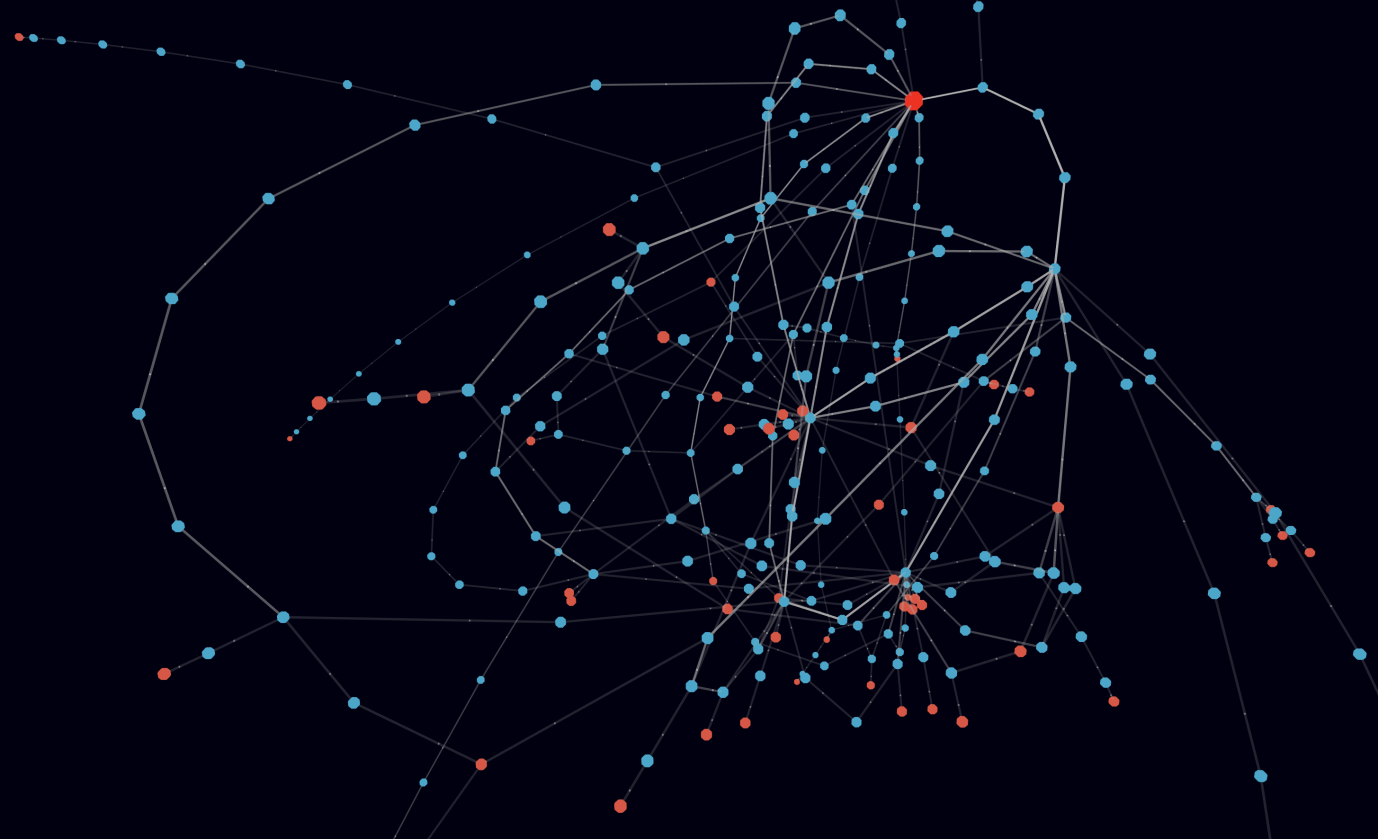
Diagram-9: Large Scale Network Formation by Ultipa Graph in Real-Time

Performance is definitely a first-class citizen on graph databases like Ultipa Graph, but that is not to ignore another first-class citizen – language intuitiveness, which requires little cognitive effort. Most people would find uQL extremely easy to ramp up with, they usually can start writing their first lines of code within 30-minute after reading the language guide.

uQL adopts chain-query practice, it’s not unfamiliar to programmers who have experience with the popular document database -- MongoDB. A typical simple chain query is like this:

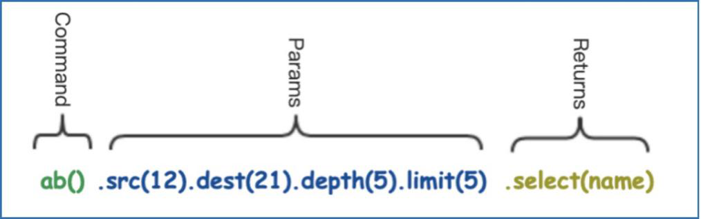
And, things can get a little bit complicated with template, which deserves some basic annotation: n() and e() refer to node and edge respectively; (a) and (b) refer to aliases that will be used in the return() clause, which is similar to SQL.

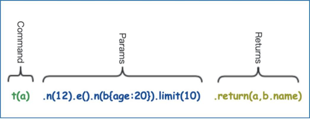
The above line of a query is to search path(s) from node=12 to ending node(s) that have attribute age=20 via any connecting edge, and return all the paths and matching ending nodes names respectively.

The next query shows the semantically recursive power of graph query, note the [3:7] part, which denotes that the query’s path search depth is between 3-hop and 7-hop inclusive:

t(a1).n(n1{age:20}).e(e1{rank:[20,30]})[3:7].n(n2).limit(5).return(a1, n1, e1, n2._id, n2.name)

This kind of flexibility is hard to achieve with regular SQL without programmatically writing a large chunk of SQL or ODBC code; besides, searching this deep on a relational database would drain all system resources and cause seg-fault.

3. Statistical queries like count(), sum(), min(), collect(), and etc.

Here is one fun example that most SQL lovers would find resonating: Calculate the sum of salaries of a company (node id=12)’s employees.

t(p).n(12).le({type:"works_for"}).n(c{type: "human"}).return(sum(c.salary))

Here is the breakdown of the above line of code:

• Putting company node as the starting node;
• Following left-pointing edge which has a relation type 'works_for';
• Searching for ending nodes with type 'human';
• Sum all end nodes' salary attribute up, and return.

In a relational database, you can do this simple example with one line of code, but it's very likely that the performance is much slower due to potential table scans on a large Employee table with tens of millions of rows.

The next example solves the problem of identifying unique provinces that the employees of a company (node id=12) are from:

t(p).n(12).e({type:"works_for"}).n(c{type:"employee"}).return(collect(c.province))

The above examples show that graph queries are capable of relational SQL queries.

And, the next 2 examples demonstrate graph queries can return results in a table-friendly way (see Diagram-10-1 and Diagram-10-2).

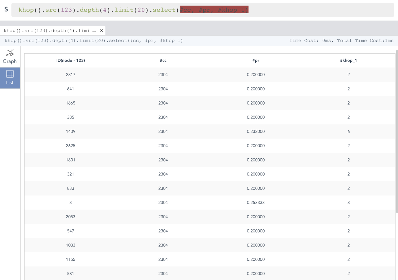
Diagram-10-1: Showing Query Results in Table Format (Ultipa Manager)

In Diagram-10-1, the khop() function is to search for vertices that are depth() away from the beginning node, and the select() function allows you to only return certain specified attributes.

The above diagram shows how the web-based Ultipa Manager presents the uQL results in a tabular/listing format. And the below diagram shows what it is like to execute the uQL command and expect the results in Ultipa CLI.

Note that there are 'Time Cost' indications on both interfaces. We mentioned that data can be tiered in terms of storage strategies, the Engine/Time Cost is the turn-around time for in-memory computing, and the Total Time Cost also includes necessary id-to-name translation time.

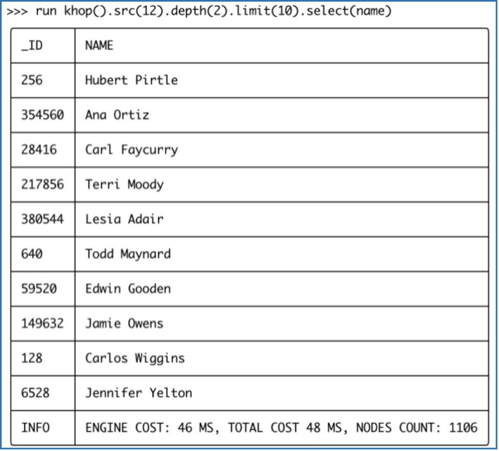
Diagram-10-2: Graph Query Results in Ultipa-CLI

4. Powerful Template-based Full-Text Search:

It would be ironic and a major lacking if the full-text search is NOT supported. Full-text search atop graph database has been around for years, like Cypher queries by Neo4j, which supports node-based full-text query; in uQL, it can be written like this:

find().nodes(~name:"Sequoia*").limit(100).select(name,intro)

The above uQL is to query for company nodes that are named 'Sequoia*', and return 100 matching nodes with node properties name and intro. This query is very much SQL-like and compatible. Similarly, you can fire the following edge-oriented full-text search:

find().edges(~name:"Love*").limit(200).select(*)

And, this simply searches for full-text indexed relationships that contain 'Love*'.

Of course, our full-text adventure won't stop here. At Ultipa, we trail-blaze a lot of things, therefore the template-based full-text search is invented to solve previously un-imaginable and daunting tasks, such as: Vaguely search for companies named 'Sequoia*', find paths that are 5-hop/layer deep to another set of companies named 'Bank*', return a certain number of resulting paths. The said question is basically to map out and formulate a complex network containing 2 sets of business entities:

t().n(~name: "Sequoia*").e()[:5].n(~name: "Bank*").limit(20).select(name)

Imagine how you would do this without uQL? On those popular online service platforms like Tian-yan-cha or Qi-cha-cha, you can find a handful of companies named 'Sequoia*', and another set of companies named 'CMB*', but to find out any in-direct connections between them is an extremely time-consuming and laborsome challenge. You either do this manually for days to possibly find a path or two or if you are the technical kind and determined to be technical to code some program to recursively search for 20 paths with end nodes that are 5-hop apart. Neither of these can beat the above uQL in terms of:

• Efficiency and Latency:  It’s done in genuine real-time;
• Efficacy and Accuracy:   The query is clear humanly easy to digest.

The beauty of an advanced query language is best manifested, not in its complexity, but in its simplicity. It should be easy to understand, therefore requiring minimum cognitive loading, and it should be lightning fast. All the real, tedious, and formidable complexities should be shielded off by the underpinning system. It’s like the ancient Greek titan Atlas carrying the world on his back, and not to burden the users of the query language and the database.

5. Complex algorithms:

Graph database has some unique features that tend to help itself gain edges over other databases, integrated algorithm functionality is one. There are many types of graph algorithms like centrality, ranking, propagation, connectivity, community-detection, graph embedding/GNN, and others. As the industries are moving forward, we may very well see more algorithms being ported over and supported by graph databases.

Taking Louvain Community Detection as an example, this algorithm recursively iterates through all vertices and edges in the graph until they find (or fail to find) communities by grouping certain vertices together (as communities). This recently invented algorithm is popular in the Internet and fintech domains. The below line of simple graph query does it all:

algo().louvain({phase1_loop:5, min_modularity_increase:0.01})

The style of invoking graph algorithm is similar to making an API call by providing necessary parameters. Not to dilute the message of simplicity, Louvain is usually time-consuming and computationally intense, the original Louvain algorithm is a sequential one, if you run it with Python’s NetworkX library, it may take many hours to finish, but with Ultipa’s unprecedented highly parallel computing engine, this is done in real-time! We are talking about performance gains of tens of thousands of times (see Diagram-11)!

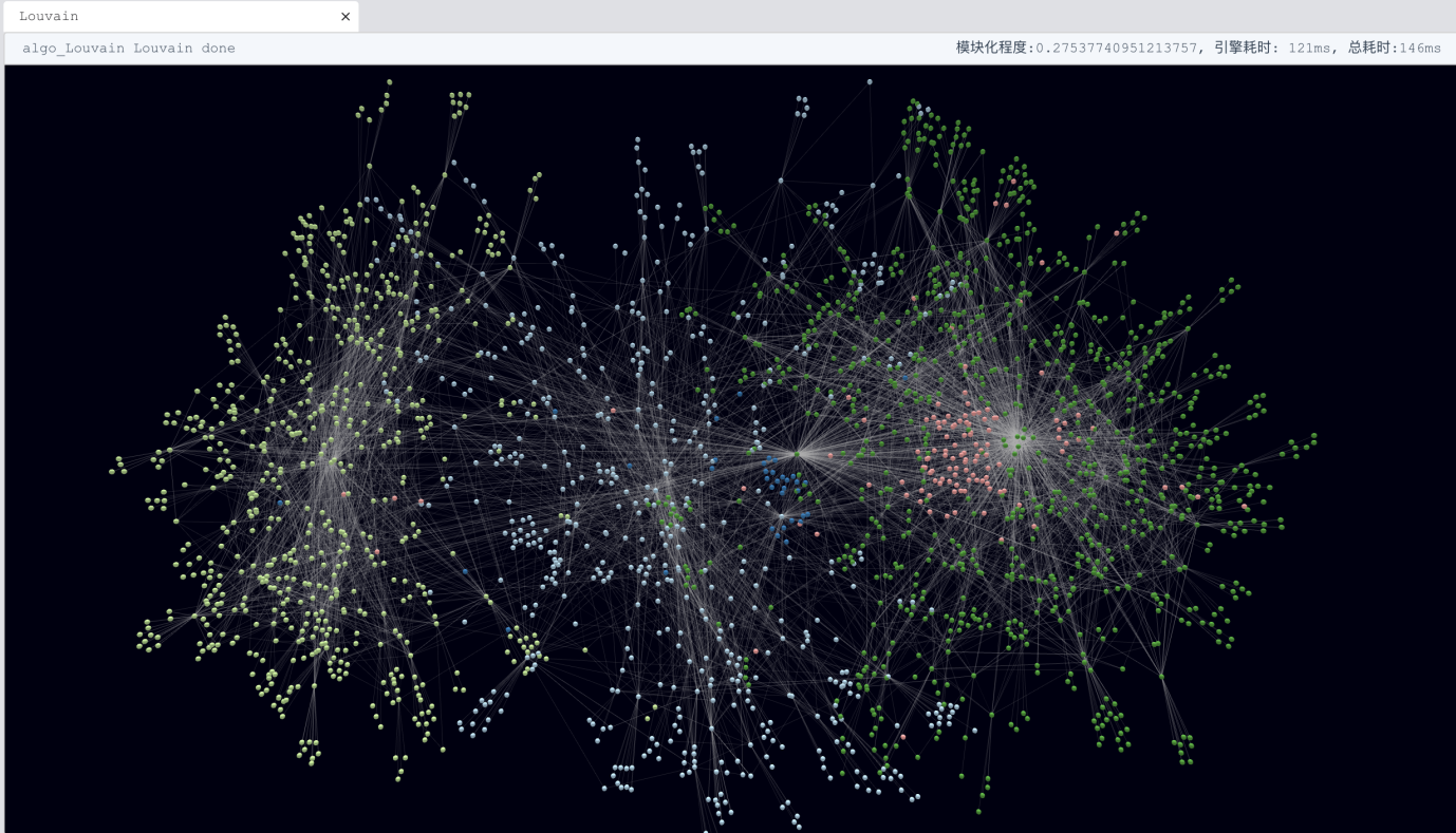
Diagram-11: Real-time Louvain Community Detection with Ultipa Manager (Web)

We hoped that the above exemplary graph queries can show that database query languages should be as simple as possible. Writing tens of or even hundreds of lines of SQL code has aggravated cognitive load. The concept we believe in is that:

• Anyone who understands business can master a database query language, not necessarily a data scientist or analyst;
• The query language should be extremely easy to use, and all the complexities are embedded within the underlying database, and transparent to users.
• Lastly, graph database has the huge potential to carry on and replace a significant share of the SQL workload, some big-name companies such as Amazon and Microsoft are speculating 40-50% SQL workload to be handled by graph databases in 8-10 years, we’ll see.  

Some people have claimed that RDBMS & SQL will never be replaced, we found this hard to believe. RDBMS replaced navigational databases in the 70s and has been rather successful for almost 5 decades, but if history has taught us anything, it is that the obsession with anything will not last forever, and this is especially true with the world of the Internet and Technologies.