By Ricky Sun

Graphs are used to represent real-world applications, especially when these applications are best represented in the form of networks, from road networks, telephone or circuit networks, power grids, and social networks to financial transaction networks. If you have not worked in a relevant domain, you may be surprised by how widely graph technologies are used. To name a few top-notch tech giants that live on graphs:

• Google: PageRank is a large-scale web-page (or URL if you will) ranking algorithm, which got its name from Google’s founder Larry Page.
• Facebook: The core feature of Facebook is its Social Graph, the last thing that it will ever open-source will be it. It's all about Friends-of-Friends-of-Friends, and if you have heard of the Six-Degree-of-Separation theory, yes, Facebook builds a huge network of friends, and for any two people to connect, the hops in between won't be exceeding 5 or 6.
• Twitter: Twitter is the American (or worldwide) edition of Chinese Weibo (and you can say the same thing that Weibo is the Chinese edition of Twitter), it ever open-sourced FlockDB in 2014, but soon abandoned it on Github. The reason is simple, though most of you open-source aficionados find it difficult to digest, that is, graph is the backbone of Twitter's core business, and open-source it simply makes no business sense!
• LinkedIn: LinkedIn is a professional social network, one of the core social features it provides is to recommend a professional that's either 2 or 3-hop away from you, and this is only made possible by powering the recommendation using a graph computing engine (or database).
• Goldman Sachs: If you recall the last worldwide financial crisis in 2007-2008, Lehman Brothers went bankruptcy, and the initial lead was Goldman Sachs withdrawing deals with L.Brothers, the reason for the withdrawal was that Goldman employs a powerful in-house graph DB system – SecDB, which was able to calculate and predict the imminent bubble-burst.
• Paypal, eBay, and many other BFSI or eCommerce players: Graph computing is NOT uncommon to these tech-driven new era Internet or Fintech companies – the core competency of graph is that it helps reveal correlations or connectivities that are NOT possible or too slow with traditional relational databases or big-data technologies which were not designed to handle deep connection findings.

The below diagram (Diagram-0) shows a typical social graph network. It was dynamically generated as an instant result of a real-time path computing query against a large graph dataset. The green node is the starting node and the purple node is the ending node, there are 15 hops in between the pair of nodes, and over 100 paths are found in between. Along each path, there are different types of edges connecting the adjacent nodes, with edges colored differently to indicate different types of social relationships.

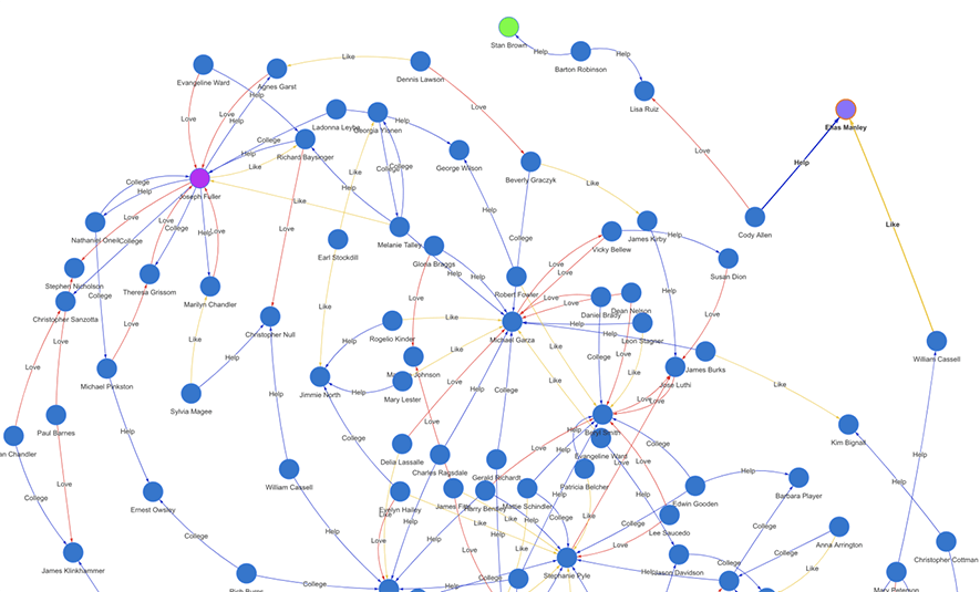
Diagram-0:  A Typical Social Graph

Graph data structures consist of 3 main types of components:

1. A set of vertices that are also called nodes;
2. A set of edges where each edge usually connects a pair of nodes (note there are more complicated scenarios that an edge may connect multiple nodes which are rare and not worth expanded discussion here);
3. A set of paths which are a combination of nodes and edges, essentially, a path is a compound structure that can be boiled down to just edges and nodes, for ease of discussion, we’ll just use the first two main types: nodes and edges in the following context.

Graph data representations:

1. Vertex:  u, v, w, a, b, c…
2. Edge: (u, v)
3. Path: (u, v), (v, w), (w, a), (a, j)… …

Note that an edge in the form of (u, v) represents a directed graph, where u is the out-node, v is the in-node. A so-called undirected graph is best represented as a bidirectional graph, that is to say, that every edge needs to be stored twice (in a bidirectional way). For instance, we can use (u, v, 1) and (v, u, -1) to differentiate that u→v is the original and obvious direction, and v←u is the inferred and not-so-obvious direction. The reason for storing bidirectionally is that: if we don’t do it this way, we’ll not be able to go from v to u, which means missing or broken path.

Traditionally, there are two main data structures to represent graphs:

1. Adjacency Matrix
2. Adjacency List

In short, the Adjacency Matrix is a square matrix, or in computer science language, a two-dimensional array, each element in the matrix indicates whether the pair of vertices are adjacent or not in the graph.

Adjacency List represents a graph in a hugely different way. It’s a collection of usually unordered lists, with each list linking all adjacent vertices to the current vertex.

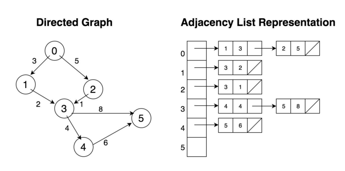
Diagram-1: Adjacency List for Directed Graph

Let’s take a deeper look at both data structures. Assuming we have a weighted graph as shown in Diagram-1, with 6 nodes and 7 edges. To represent in an Adjacency Matrix, each element in the graph (as in Diagram-2) indicates if an edge exists between any two vertices. Clearly, the matrix is sparse, the occupation rate is (7/36) <20%; however, the storage space required is 36 bytes if each element takes 1 byte. If there are 1 million vertices in the graph (which is a pretty small graph in the real business world), the storage space needed is 1M*1M = 1 trillion bytes = 1000GB.

Diagram-2: Adjacency Matrix for Directed Graph

People may argue that the above calculations are exaggerated, and we will show how it is not. Yes, if each element can be represented using only 1 bit, the aforementioned 1M*1M graph storage can be shrunk to 125GB. However, we were talking about a weighted graph, and each element needs at least a byte to represent the edge’s weight; and if there are additional attributes, the matrix simply grows larger, therefore, seeing the need for storage space beyond control.

Modern GPUs are known for matrix-based computations, and they usually have a restriction on the size of the graphs: 32,768 vertices. This is understandable because the graph with 32K nodes represented in the Adjacency Matrix data structure would occupy 1GB+ RAM, which is 25-50% of a GPU’s RAM limit. Or, in another word, GPUs are not suitable for larger graph calculations, unless you go through the painful and complicated process of graph partitioning (or sharding).

Storage inefficiency is the biggest foe against Adjacency Matrix, that’s why it’s not a popular data structure beyond academic researches. Let’s examine the Adjacency List next.

As illustrated in Diagram-1, the Adjacency List represents a graph by associating each node with a full collection of its neighboring vertices. And, naturally, in its original design, each element (node) in the linked list together with the header node form an edge connecting the two nodes.

Adjacency List is widely used, such as in Facebook’s core social graph, a.k.a Tao/Dragon architecture design. Each vertex represents a person, and the linked list behind the vertex is the person’s friends or followers.

This design is easy to understand and storage-wise efficient; however, it may suffer from hot-spot operational problems. For example, if there is a vertex with 10,000 neighbors, the linked list is as deep as 10,000 steps, to traverse the list, the computational complexity in big-O notation is O(10,000). Operations like Deletion, Update, or simply Read take an equally long time (or on average a latency of O(5,000)). Also, linked-list is NOT concurrency friendly, you can’t achieve parallelism with a linked-list!

These concerns put the Adjacency List in a disadvantageous spot compared with the Adjacency Matrix, which takes a constant O(1) time to update, read or delete.

Now, let’s consider a method, a data structure that can balance the following two things:

• Size: Storage space need
• Speed: Latency of access (and concurrency friendliness)

The size part is obvious that we try not to use a sparse data structure with lots of empty elements thus wasting lots of precious RAM space (we are talking about real-time in-memory computing if you will), and the core concept of Adjacency List serves this size reduction purpose well; the only caveat is that the naming can be misleading – we want a non-list-centric data structure!

Here we come up with a new name, a new data structure, adjacency hash<*>. Search for a vertex takes a constant latency of O(1), and locating a particular edge (the in-node and the out-node) takes only O(2), assuming a way of accessing the element via subscript (index). This can be implemented with an array of vectors as in C++.

// Array of vectors

Vector <pair<int,int>> a_of_v[n];   

A typical implementation of the high-performance single-threaded hash table is Google’s SparseHash library which has a hash table implementation called dense_hash_map. C++ 11 also has unordered_map implementation, a chaining hash table that sacrifices memory usage for fast lookup performance. The problems with these 2 implementations are that they don’t scale with the number of CPU cores – meaning only 1 reader or 1 writer is allowed at the same time.

In a modern, cloud-based high-performance computing environment, superior speed can be (ideally) achieved with parallel computing, which means having a concurrent data structure that utilizes multiple-core CPU and even to the extent of enabling multiple physically or logically separated machines (computing nodes for instance) to work together against a logically universal data set. 

Traditional hash implementations are single-thread/single-task oriented, meaning that a second thread or task which competes for common resources would be blocked.

A natural extension would be implementing a single-writer-multiple-reader concurrent hash, which allows multiple readers to access critical (competing) data sections concurrently; however, only 1 writer is allowed at a given time to the data section.

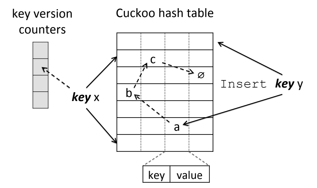
Diagram-3: Hash Key Mapped to Two Buckets and One Version Counter

Single-writer-multiple-reader designs often use techniques like versioning or read-copy-update (RCU), which is popularly seen in Linux Kernels. There are other techniques like open-addressing and etc. MemC3/Cuckoo hashing is one such implementation (See Diagram-3).

Leaping forward, ideally, we would want multiple-reader-multiple-writer concurrency support; but this would seemingly be in direct contradiction with the ACID requirement, especially the strong need for data consistency in business environments when you think multiple tasks or threads accessing/updating values at the same time to realize so-called scalable concurrent hashing.  

To realize 'scalable concurrent hash data structure', we must evolve the adjacency hash<*> to be full-concurrency capable. There are a few major hurdles to overcome:

• Non-blocking and/or Lock-free
• Fine-granularity access control

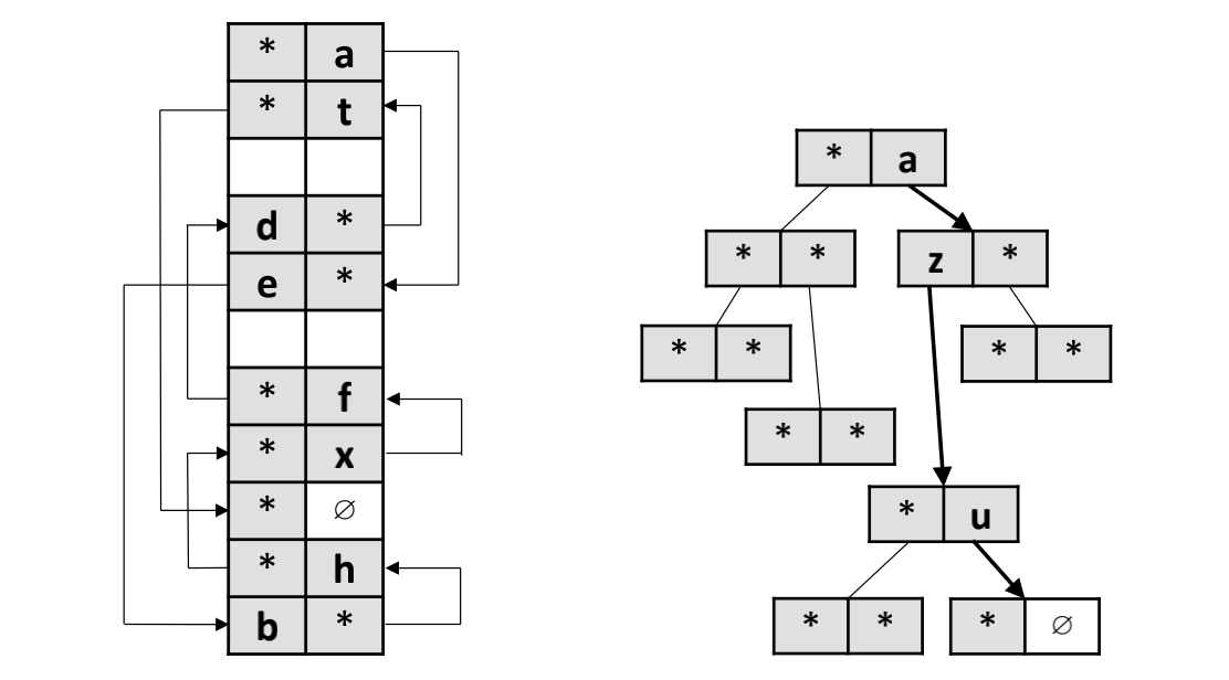
Diagram-4: Random Placements vs. BFS-based Two-way Set-Associative Hashing

To overcome the aforementioned hurdles, both are highly related to the concurrency control mechanism, a few priorities to consider:

• Critical Sections:
  • Size: Kept minimal
  • Execution Time: Kept minimal
• Common Data Access:
  • Avoid unnecessary access
  • Avoid unintentional access
• Concurrency Control
  • Fine-grained locking: lock-striping, lightweight-spinlock
  • Speculation locking (i.e., Transactional Lock Elision)

The bottom-line of a highly concurrent system is comprised of the following characteristics:

• Concurrency-capable infrastructure
• Concurrency-capable data structures
• Concurrency-capable algorithms

The infrastructure part encompasses both hardware and software architectures. For instance, the Intel TSX (Transactional Synchronization Extensions), which is hardware-level transactional memory support atop 64-bit Intel architecture. On the software front, programs can declare a section of code as a transaction, meaning atomic operation for the transactional code section. Features like TSX provides a speedup of 140% on average.  

On the other hand, with a concurrency-capable data structure (which is the main content of this article), you still have to write your code carefully to make sure that your algorithm fully utilizes concurrent data processing.

The below diagram shows the performance of a high-concurrency graph computing scenario, K-HOP() operations, on Ultipa Server, which is powered by Ultipa Engine, a high-performance real-time graph computing engine.

K-Hop is to calculate the set of neighbors that are exactly K hops away from the starting vertex. And the number of hops is the length of the shortest paths between the starting vertex and any vertex in the resulting set. K-hop is usually calculated in a BFS manner.

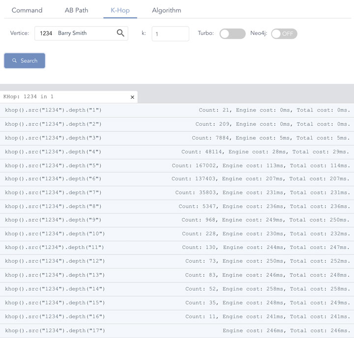
Diagram-5: Ultipa Real-Time Deep Graph Traversal with Concurrent Hashing

BFS is one of the easier ones to achieve concurrency, compared with DFS and other more complicated graph algorithms (i.e., Louvain Community Detection). The below diagram (Diagram-6) shows how we compute concurrently.

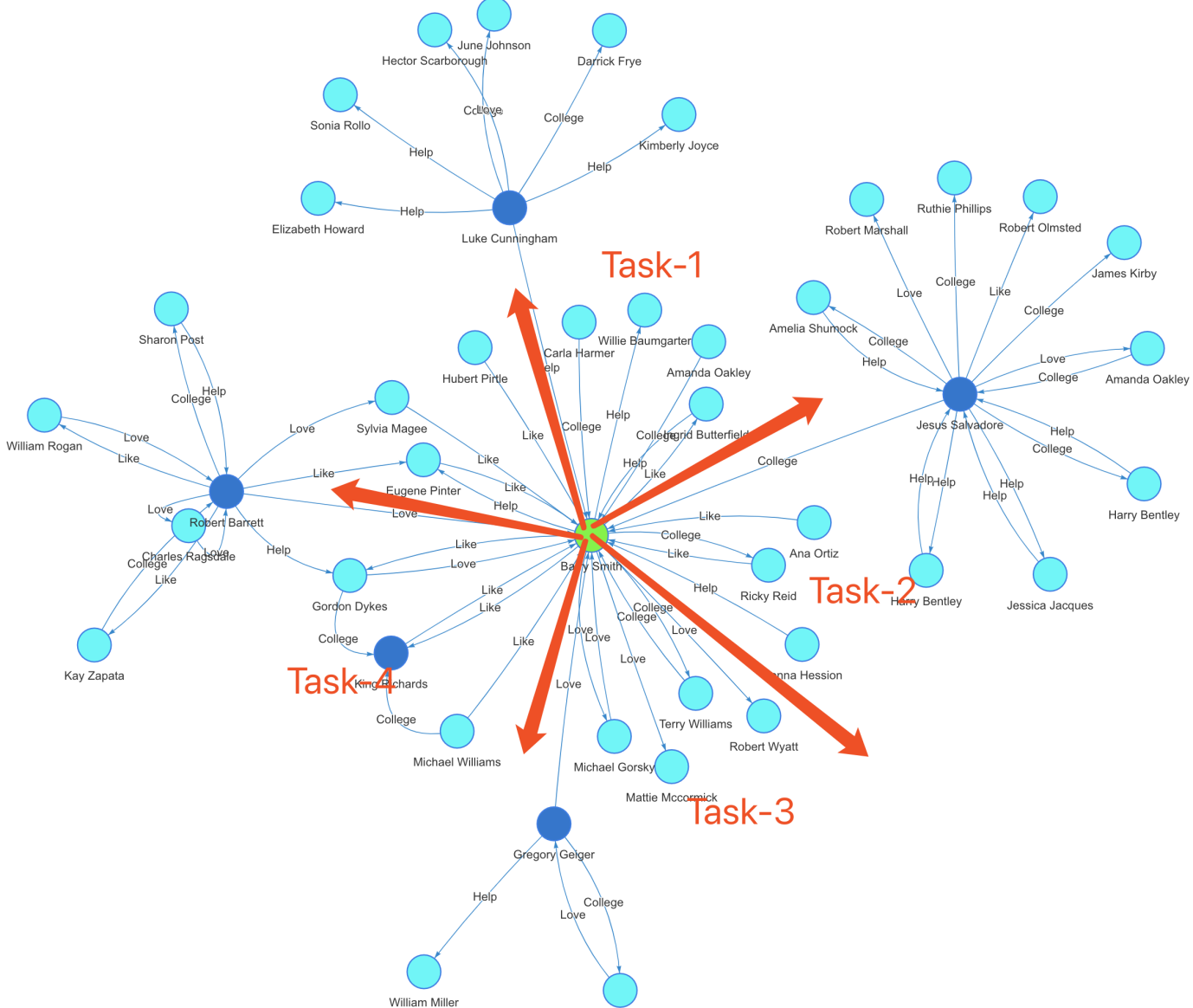
Diagram-6:  K-hop Concurrency Algorithm

K-Hop Concurrency Algorithm:

1. Locating the starting vertex (the green node at the center), determining how many unique adjacent nodes it has, if K==1, return directly with the # of nodes, otherwise, proceed to step-2.
2. K>=2, determine how many threads of tasks we can allocate for concurrent computing, divide the nodes from step-1 into each task and continue to step-3.
3. Each task further divides and conquers by calculating adjacent neighbors of the node in question and proceeds in a recursive way until there are no further nodes to calculate upon.

The testing dataset is Amazon-0601 which has half-million vertices and 3.5 million edges. This dataset is commonly available for graph benchmarking and is considered a small-to-medium size in industrial circumstances (Note: this is unlike academic circumstances that usually work on relatively small datasets).  Based on the aforementioned algorithm, in Diagram-5, the engine runtime for 1-hop and 2-hop are well below 1 millisecond (completed in microseconds scale), starting from 3-hop, the resulting numbers are edging up quickly,  computationally the complexity is exponential, but with sufficient concurrency, the latency maintains low and even sub-linear – this is reflected in hop-depth from 6 to 17.

But if you do an apple-to-apple comparison, taking Neo4J as an example, 1-hop takes 202ms, which is about 1,000 times slower, and starting from 5-hop things are getting much slower (exponentially slower which effectively makes it impractical to operate anymore).

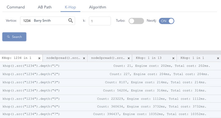
Diagram-7: Neo4J’s Performance on Graph Traversal

For graph search depth>=8, Neo4j never returns. More importantly, Neo4j’s K-hop calculations are bluntly wrong on all hop depths >=2. For instance, in 2-hop, the results 227 includes some nodes from 1-hop, this is because Neo4j’s graph engine does NOT de-duplicate and might be using wrongful BFS implementations as well.

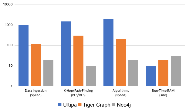
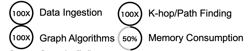
Diagram-8: Ultipa 2D vs. 3D 1-to-K Hop Expansion

As a side-note, visualization is all-important with graph database, and since graph is very much high-dimensional compared to relational DBMS’ 2-dimension table-row-column setup, it would make every sense to visualize the results, make it highly explainable (the meaning of white-box AI!) and allow users to interact with the data with ease. Diagram-8 shows the 2D and 3D GUI of Ultipa Manager (Ultipa Server’s front-end and operational center).

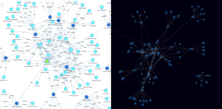
Diagram-9: Performance Comparison of Ultipa vs. Neo4J vs. Tiger Graph

To recap on the evolution of graph data structure, there are opportunities to achieve higher throughput via concurrency almost encompassing the entire life-cycle of data, ranging from:

• Data Ingestion
• Data Computations from K-hop to Path-query and more
• Batch-processing Algorithms

Additionally, memory consumption is a storage factor to consider. Even though we all proclaim that memory is the new disk and it offers far superior performance to disks (SSD or magnetic), it’s not boundless, and it is more expensive, using it with caution is a must-have. There are valuable techniques to reduce memory consumption:

• Data Modeling for Data Acceleration
• Data Compression & De-duplication
• Choosing Algorithms or Writing Code that Do NOT cause bloat

Hopefully, you have enjoyed reading this article so far, in the next article, we will be covering techniques on data-processing acceleration, please stay tuned.