By Ricky Sun, Jason Zhang, and Victor Wang

Part-I

We have learned that relational databases use SQL and two-dimensional tables to model after the world, this is in deep contrast to how graph databases address the problem. In short, graph databases use high-dimensional data modeling strategies to 100% resemble the world – and because the real world is highly dimensional, graph is considered 100% natural. This naturalness comes with a challenge, especially for people who are accustomed to the trade-off hypothesis or the zero-sum game theories. The challenge is that you have to be brave enough and smart enough to think out of the box and the limiting belief that 'There is no better way of modeling the real-world problems beyond SQL or RDBMS'.

In our previous essay on The Evolution of Database Query Languages, we depicted the evolution of SQL and NoSQL, and their advantages and disadvantages. In today’s business world, we are seeing more and more businesses relying on graph analytics and graph computing to empower their business decisions.

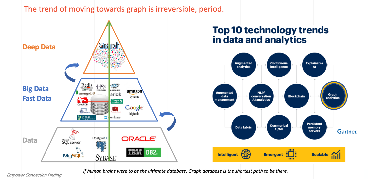
Graph-0 Deep Data and Graph Analytics – A Major Trend in202x

In a series of reports from November 2019 to June 2020, Gartner predicted that Graph analytics is not only 1 of the top 10 Data & Analytics trends (see the above diagram), but also laid out that: By 2025, 80% of business intelligence innovation worldwide will be powered by graph analytics.

Now, let’s pause for a second and ponder on the top features you would desire graph databases to offer. What are they? This is a question equivalent to asking: What features are missing in SQL and RDBMS?

As always, this is an open question and the answer can be highly diversified and warrants no standardization. However, out of all possible answers, 3 things come out of our guts feeling and if you think deeply, you will resonate with us, they are:

• Simplicity (i.e., Enjoy writing 100s of lines of SQL?)
• Recursive Operations (i.e., Recursive Queries)
• Speed (i.e., Real-time-ness)

In a reversed order, let’s go through this 3-strike-out list.

Speed

In a reversed order, let’s go through this 3-strike-out list: Speed and lightning fast performance is deeply rooted in the original promise of what graph database offers to the world. Because conventional table joins are insanely slow to churn out data due to the well-known cartesian-product or table-scan problem, a fundamental change of the way we model and process data therefore is both necessary and pivotal.

If you think from the high-dimensional space, graph is the most natural way to connect the dots (vertices) by connecting entities into a network, a tree or a graph, and working against the graph is simply to find the neighbors of any vertex, paths reaching to or leaving from the vertex, common attributes sharing between any pair of vertices (similarity), centrality of a graph or sub-graph, ranking of a vertex in the graph, and etc.

There are many ways to work against the graph and sought for values out of it. However, as the graph is getting larger, denser or the queries are getting more sophisticated, the performance degradation is considered a norm by most people… Well, this doesn’t have to be so.

Consider the following scenario: In a social graph of millions of users who interact with each other, find 200 pairs of users (starting from users whose age=22, ending with users age=33) who are 1-hop to 10-hop away from each other. Gauge the performance degradation, if there are any.

Graph-1 Real-Time Deep Graph Traversal by Ultipa Graph

The above screenshots show the turn-around time (roundtrip latency) of running the queries on Ultipa Graph (a high-performance graph database that’s capable of real-time ultra-deep graph traversal) against a reinforced Amazon-0601 Graph Dataset (3.5 Million Edges and 0.5 Million Vertices with multiple attritubtes like id, name, age, type of relationship, rank, and etc.). These queries traverse the graph based on the template path query criteria, starting from 1-hop, gradually going deeper to 20-hop. The following chart captures the query latency comparison:

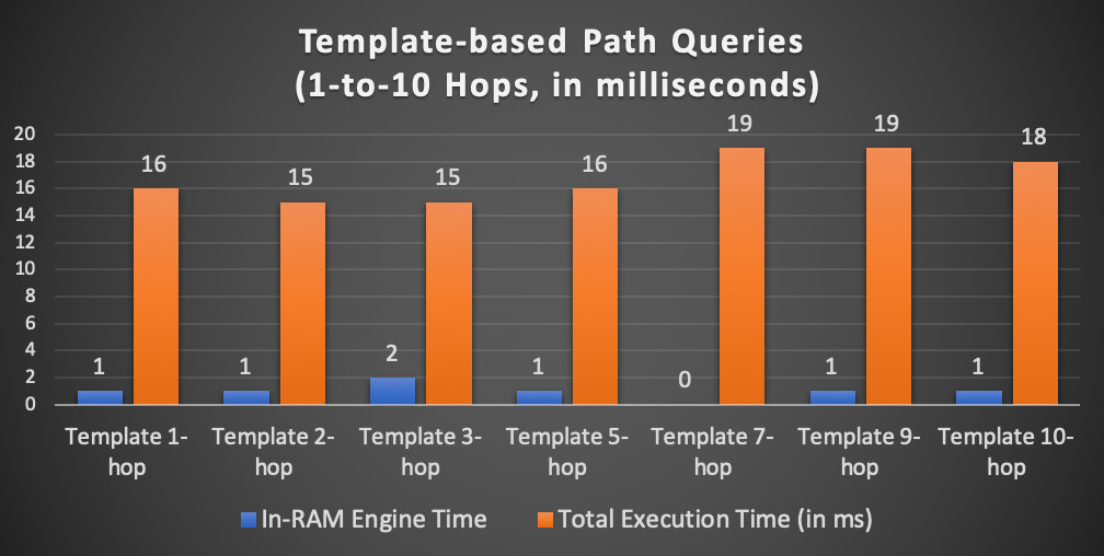
Graph-2 Graph Traversal Latency & Breakdown (Ultipa Graph)

As you can see that when we are traversing deeper into the graph, the overall latency growth trend stays flat or sublinear instead of being exponential. There is no obvious  performance degradation. If you think about locating 200 paths in a graph, each with a formidable lenth of 20 (20 edges and 21 vertices along the path), plus the filtering parameters of starting users having age=22, ending users age=33, the complexity of such kind of queries is pretty formidable.

This almost flat, definitely sublinear, query latency growth is achieved with 3 core technologies as illustrated in the below diagram:

• High-Density Parallel Graph Computing
• Ultra-Deep Graph Traversal (and Dynamic Graph Pruning)
• Multi-layer Storage and Computing Acceleration

And, they jointly and interwovenly bring about 3 major benefits:

• Faster Time-to-Value and Time-to-Market
• Much Lower TCO
• Superb Usability and user experience

 Graph-3 Core Advantages of Ultipa Graph (3x3)

Graph DBMS, unlike realtion DBMS, NoSQLs or Hadoop/Spark, scales out differently. The key difference lies with graph’s unique strength: Its ability to process data wholistically. In another word, graph DBMS must allow deep penetration (and correlation) of data, while all other RDBMS, NoSQL or Big Data frameworks do NOT have similar capacity. To draw an analogy in the context of RDBMS/SQL, to deeply penetrate data is to have multiple tables join together, and this can be disastrous.

Graph-4 Cartesian Product of Multi-Table Join

Graph-4 illustrates this problem: when 2 tables are joining together, the cartesian-product effect will create a large tables that multiplies rows of both tables together. If there are multiple large tables (i.e., millions of rows) involved, the size of the resulting table can be outrageous, and this outrageousness means it’s impossible to get your query results in real-time, not only that, practically speaking, you can’t even get a result in time.

In Graph-5, we illustrate that a typical attribution analysis (a.k.a., contribution analysis or performance/impact analysis) using SQL/RDBMS would need 1,000 server’s 10-day’s computing time and tons of storage to calculate all possibilities, the sheer computing complexity by SQL/RDBMS is unbearable, they are too rigid, too slow, and too complex.

A paradigm shift is due to happen and it’s graph computing and graph database coming to the rescue. Graph-6 illustrates the difference between a typical realtional database and a graph system, as we are digging deeper (more hops) into data, the latency grows exponentially with realtional DBMS, but linearly with graph DBMS. This makes all the differences.

Graph-5 Astronomical Computing Complexity with SQL/RDBMS and DW

Graph-6 The Paradigm Shift by Graph Computing

There are graph vendors out there promoting unlimited scalability graph DBMS that’s capable of a single graph with trillions of vertices and edges. We found this to be a myth. And there are 2 points to bust this myth:

• In what scenarios you have to use a single graph with trillions of vertices/edges? A trillion-scale graph must be disseminated into many physical instances, for any query that requires processing against all instances while they all depending on each other for intermediate results will exponentially slow down the overall system performance, this is a typical dilemma of any BSP (Bulky Synchronous Processing ) system. Can you imagine how slow a large BSP system can be if you ask it to handle 3-hop or deeper graph queries?
• A wiser design of a horizontally distributed graph DBMS is to orchestrate a system that contains multiple (or many) graphs. Just as you would for a RDBMS with many tables. Typical scenarios like financial transactions, which tend to have timestamps, and you can logically disseminate one year’s transactions into 12 months, and each monthful transactions can be self-contained within a single graph (essentially connecting all transacting accounts with transactions that happen in the current month), and jointly, 12 months’ worth of graphs constitute a logically complete jumbo graph.

The points above paragraph should remind the readers who wonder why JanusGraph, AWS Neptune or ArangoDB (and a handful other commercial graph products) are so sluggish and can NOT return in a timely fashion while trying to accomoplish the same kind of graph queries. Their core weakness lies in their unwise and blindly complicated distributed architecture design.

Putting distribution strategy aside, the most important techniques to accelerate graph queries (like path-finding or k-hopping) are through high-denisty computing and deep-traversal-n-runtime-pruning.  However, these 2 supposedly fundamental techniques are long forgotten by many programmers. Admittedly, we are living in a world of high level programming languages, millions of newer generation young programmers are believing that the omni-potent power and ease of Python is ruling the world. However, in terms of processing power, it’s simply problematic, so is Java and any languages that dwell on GC (garbage collection).

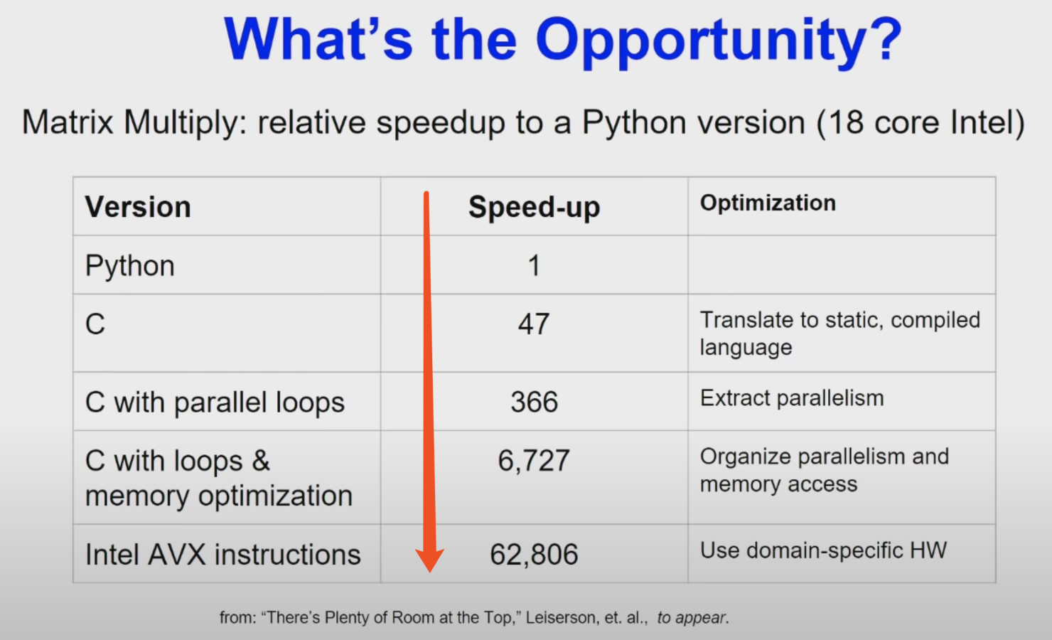
Graph-7 Parallel Architecture Design and Memory Optimization (Turning Lecture 2018)

In ACM’s 2018 Annual Turning Lecture , Turing Award recipients David Patterson and John Hennessy outlilned the opportunity to speed up Python program using parallel C on 18-core Intel X86-64 CPU by over 62,000 times! It’s achieved with:

• Lower-level Programming Language (to maximize HW juice)
• Memory Optimization (ditto)
• Leverage CPU’s Advanced Instruction-Set Features (ditto)

All in all, these techniques are all contributing to the realization of “high-density” computing. Moreover, runtime dynamic graph pruning and deep graph traversal are realized with novel data structure design. In a previous essay by the authors titled The Specific Evolution of Graph Data Structures,  a novel Adjacency Hash* data structures were introduced and can be used effectively to store graph topology and enable runtime filtering (a.k.a dynamic graph trimming or pruning) – of course, the most dramatic part is that: Most majority of the operations on the graph are having a big-O notation, in terms of time complexity, of O(1) – instead of O(log N) or O(N) or even O(N * log N) ... This is critically important to ensure that when we traverse the graph deeply, we won’t have to deal with the exponentially growing search complexities. Here is an outline of the “Exponential Challenge”, taking the boosted Amazon-0601 Graph Dataset as an example.

• |E|/|V| = 8 (average degree of vertex)
• Complexity of Searching 1-hop paths ~= 8
• Complexity of Searching 2-hop paths ~= 64
• Complexity of Searching 5-hop paths ~= 8*8*8*8*8 = 32,768
• Complexity of Searching 10-hop paths ~= 1,073,741,824 (1Billion Searches)
• Complexity of Searching 200 pairs of 10-hop paths ~= 200 Billion!

 Clearly, if the complexity was really over 200 Billion, there is NO WAY for any graph system to return within milliseconds. The above complexity was only theoretical. In reality, the maximum possible searching complexity for an O(1) operations is by no means exceeding the total number of edges in the graph, which stands at 3.5 million in our case, therefore, we can assume that starting from 7-hop (32768 * 8 * 8) to any deeper hops, the max complexity is capped at 3.5 million (for Amazon 0601, the real complexity, in temrs of this Amazon dataset is actually caped at ~0.2 million, sepecially around 6 to 8-hop deep)

• Adjusted complexities for 6 to 10-hop paths = max 200,000 each hop.

Therefore, it’s possible to review the breakdown of the latency as in Graph-8:

Graph-8  O(1) Complexity and Latency Breakdown Chart

Comparing the numbers in Graph-8 against those in Graph-1 & Graph-2, it’s NOT hard to come to the takeaways: By leveraging maximum concurrency (parallelization) and CPU caching, Ultipa achieved latency in close proximity to underlying hardware platform’s max throughput. The same operations on any other graph databases, namely Neo4j, TigerGraph, D-Graph, ArangoDB or any other products, would take either much longer than HDD or SSD’s performance, or they could never return and drop dead due to the computational complexity of traversing 10-hop deep (TigerGraph might stand somewhere between SSD and IN-RAM, but definitely can NOT return for traversal operations deeper than 10-hop).

Part-II

Recursive Operation

We have covered the SPEED and performance part in Part-I of this series of articles. It’s time to talk about a unique feature by graph database, which really should be universally available – recursive operations during networked (linked-entity) analysis.

Graph-9  Complicated SQL vs. Simplistic GQL/UQL

Taking UBO (Ultimate Beneficiary Owner) identification as an example, regulators around the world are trying to identify the ultimate business owners who may be hiding behind layers of intermediate shell companies. On the other hand, large enterprises or individuals tend to diversify their business operations by investing in other companies which in turn further invest downstream and eventually building out a gigantic network of industrial and commercial graph (a special form of knowledge graph if you will)  with millions of companies and natural persons (individuals who are owners, stake-holders, senior management, or legal representatives).

In Graph-9, we illustrate how SQL and GQL handles UBO-identification respectively. As you can see, it is very awkward for SQL to handle recursive queries which is to start from a subject company and to trace (penetrate) upstream for stakeholders for up to five layers. You have to write many lines of SQL code, which is counter-intuitive! And, on a small table of only 10,000 rows (investment relationship), SQL needs dozens of seconds to churn out results, which means it will take forever on larger tables of millions to billions of rows.

On the other hand, writing GQL can be surprisingly straightforward. In Graph-10, an easy-to-understand one-liner was fired up from Ultipa Manager (an integrated Web-GUI for Ultipa graph database management) to query a large dataset of millions of entities for investors that are hiding 5-hop away from the subject company. The results in linked-entity format are returned in real-time with clear identification of the subject company, intermediate companies, and ultimate investors.

Graph-10  UBO Query Results Visualized in Ultipa Manager

In Graph-9 and Graph-10, we briefly illustrate the capability difference between SQL and GQL when conducting networked/linked-analysis. It’s worthwhile expanding on this topic analytically, let’s revisit our query from Part-I:

Find 200 pairs of users (starting from users whose age=22, ending with users age=33) who are exactly X-hop away from each other. Assuming X=[1-20]

From query language design perspective, how would you define and articulate the question and fetch the answer accordingly?

The key part is to make the query narrative, which means naturally resembling human language therefore easy to understand, meanwhile making it recursive and succinct so that you don’t have to labor on writing your logic in a convoluted (i.e., SQL) way.

n({age==22}).e()[10].n({age==39}) as paths return paths limit 200

Graph-11  Template-based Path Search Query and List-style Results (of Paths)

The above one liner written in UQL was pretty self-explainable, but just in case you are in shock of getting the gist of it, the recursive part lies with the e()[10], which specifies that the search depth is exactly 10-hop, of course you can modify it to be e()[5:11] which stands for traversing depth from 5 to 11-hop inclusively, or e()[:10] which means up to 10-hop, or e()[*:10]  where * stands for shortest-path (BFS) search but with max traversal depth by 10.

Of course, the query can be expanded in many ways, such as filtering by attributes on the edges, or doing mathematical and statistical calculations. For instance, searching along the path by identifying with only relationship=“Love”, the results are captured in Graph-12, with the following updated query:

n({age==22}).e({name=="Invest"})[3:5].n({age==39}) as p return p limit 200

Graph-12  Template-based Path Search Query and 2D graph-style Results (of Paths)

Simplicity

Empowered with powerful recursive queries, a lot of things can be accomplished with great simplicity. In the remaining section, we would like to draw comparisons among Neo4j, TigerGraph and Ultipa. As the Chinese saying goes: Truth comes out of comparison. Let’s reveal the truth next.

Graph-13 Comparison of Cypher, GSQL, Gremlin and UQL

In Graph-13, we compare Cypher, Gremlin, UQL and GSQL while having them describe a typical linked-data triple, where a labeled entity (Person) has a job(relation) function as a Chef (Job).  As you can clearly see, the following takeaways are listed here for review:

• GSQL is incredible complex, and for such a simple triple, it would require writing 10+ lines of code, for a real complex scenario, you just can’t imagine your coding and maintenance experience.
• Gremlin’s language design is weird, it looks both verbose and confusing, some functions can clearly be consolidated into fewer chained components.
• The main difference between Cypher and UQL lies in the Cypher still uses WHERE sub-clause as SQL does, but UQL allows this part to be done naturally inline.
• Lastly, UQL supports both schematized and schema-free, the former is to allow schematized (strong-type) matching, while the latter is more flexible to support dataset that’s not-yet-schematized. In UQL, this is called demi-schema, it offers great flexibility when dealing with heterogeneous types of data.

Most of today’s system implementing smart recommendation involve some sort of social recommendation, which was coined: collaborative filtering. The core concept is actually easy – it’s essentially “graphy”:

To recommend something, some products, to a customer, we usually first look through the customer’s friends’ shopping behavior, and recommend based on the findings…

Let’s see how the 3 graph systems tackle the collaborative filtering challenge.

Neo4j uses Cypher to write the below logic:

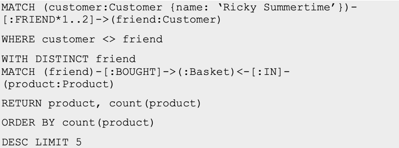
The Cypher logic goes like this:

1. Find Ricky’s friends and friends-of-friends (1^stpart)
2. Collect distinct (unique) friends
3. Find what products these friends bought (2^ndpart)
4. Return the top-5 purchased products

The Neo4j logic has a prerequisite on the dataset, it assumes that the friends type of relationship are available. This is a major assumption that most e-commerce websites can hardly satisfy, not even on the world’s largest Taobao or T-mall sites – they don’t keep track of the user’s social network information!

The other obvious limitation of Neo4j & Cypher is that it does NOT allow deep traversal on the graph, you will have to pause after searching for 1 to 2 hop deep and construct the intermediate dataset (friends), then continue with the 2^nd part of the search. This symptom can be aggravated in scenarios like UBO (Ultimate Business Owner) finding, where you need deep traversal sometimes 10 or even 20-hop deep. Neo4j can NOT handle that kind of scenario with simplicity or speed.

TigerGraph uses GSQL (short for GraphSQL) to conduct “collaborative filtering”, the below chunk of code from Tigergraph online documents illustrate how this can be done. First, supply a set of users (input_user), next, find all target users that liked the inputed users, thirdly, proceed from these target users and continue to search for users that they liked and aggregate (ACCUM) and return in ordered fashion.

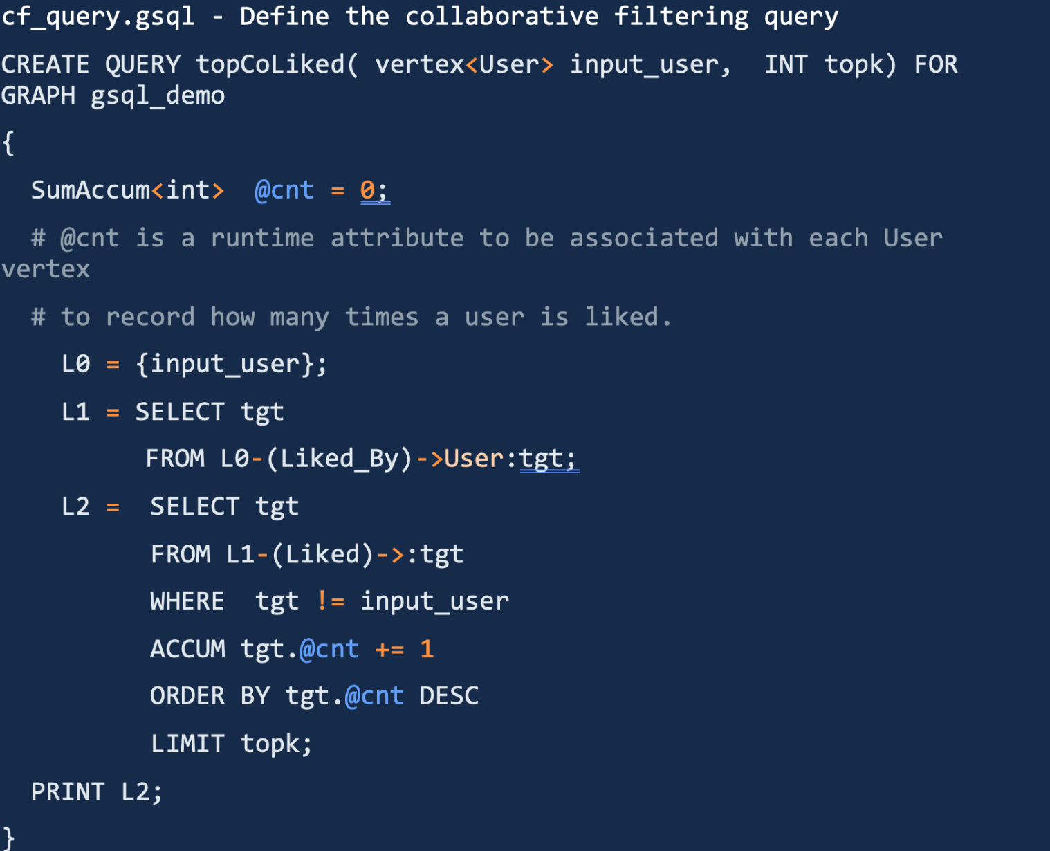
First of all, this example essentially is a 2-hop template-based path search with data aggregation. Besides, the above GSQL is way too complicated, awkward and lengthy. One key drawback about SQL is that it drains a lot of human cognition power – a SQL stored procedure longer than 10 lines is getting unbearably difficult to interpret. And this cluster of GSQL code gives us all the bad memories about SQL.

Just for the sake of comparison and show-case of simplicity, if UQL were to accomplish the same, you only need to write:

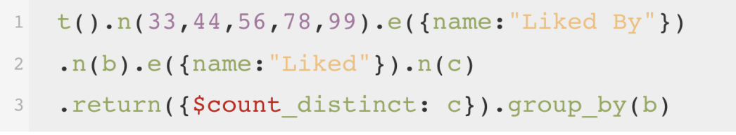
Pretty simple and straightforward, isn’t it?

• First, start a template search (t()), starting from a set of nodes n();
• Second, traverse edges named “Liked By” (or any other attribute);
• Third, continue to traverse edges typed “Liked”, reaching nodes aliased c;
• Fourth, return distinct c and group by b.

Let’s get back to our original question on collaborative filtering, on an e-commerce graph dataset, it’s comprised of customers, products and shopping or browsing behavior connecting users and products. Think in a very graphy way, you will basically need to achieve the following steps:

1. Starting from a user, find all products (viewed, added or purchased)
2. Find all users that have had certain actions (i.e., purchase) on these products
3. Find all other products that are taken actions by users in Step 2.
4. Return some of the products (i.e., top ranked) and recommend to the user.

The results are shown on the following diagram:

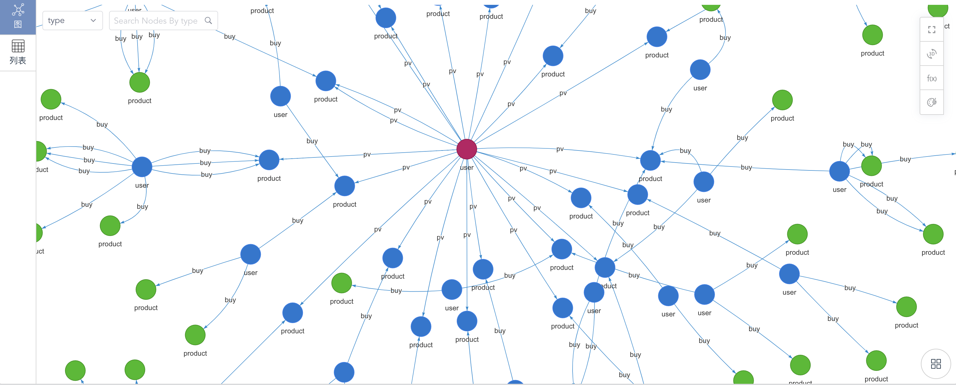
 Graph-14  Template-based Graph Query for Collaborative Filtering

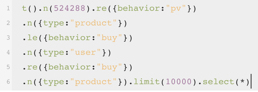
The UQL used to realize this was a template-based path query, as shown from below, which narrates the path filtering criteria as defined from above. The eventual to-be-recommended products may be further filtered, ranked or processed in a more sophisticated way, but the query language by itself is ostensibly self-evident and easy to digest:

In this series of articles, we have discussed the two key features of graph database:

• Speed: If speed and performance are not important, what else can be more important? The whole promise of graph database is rooted in unprecedented data penetration capabilities which directly translates into speed!
• Simplicity: Graph data is high-dimensional, and SQL is far from being capable of handling graph queries. If we were to design GQL, we want the queries to be humanly easy-to-digest and, of course, easy-to-code, so that secondary-development atop graph database can offer faster time-to-value and time-to-market.

The beauty of a data query language is best manifested, not in its complexity, but in its simplicity. It should be easy to understand, therefore requiring minimum cognitive loading, and it should be lightning fast! All the tedious and formidable complexities should be shielded off by the underpinning system therefore transparent to human users. It’s like the ancient Greek titan Atlas carrying the Earth on his shoulder, and not to burden the users living on the Earth (=users of the query language and the database).

Writing tens of or even hundreds of lines of SQL code has aggravated cognitive load. The concept we believe in is that:

• Anyone who understands business can master a graph database query language, not necessarily a data scientist.
• The query language should be extremely easy to use, and all the complexities are embedded within the underlying database, and transparent to users.
• Lastly, graph database has the huge potential to replace a significant share of the SQL workload, in a 2021 report by Gartner, it’s predicted that 80% of all business intelligence innovations will be powered by graph analytics by 2025, the growth trajectory of graph is exponential!

Some people have claimed that RDBMS & SQL will never be replaced, we found this hard to believe, RDBMS had replaced navigational databases in the 70s and been rather successful for almost 5 decades, but if history has taught us anything, it is that the obsession with anything will not last forever, this is especially true in the world of Internet and Information Technologies.

“What you cherish, perish”

“What you resist, persist”

If human brains were to be the ultimate database,

Graph database is the shortest path to be there.