Graph Database Benchmarks Demystified (Part 1)
June 13, 2022
Ricky Sun
Founder & CEO
Ultipa Inc.

The main goal of this article is to introduce basic knowledge about graph database, graph computing and analytics, and to help readers interpret benchmark testing reports, and to validate if the results are correct and sensible.
Basic Knowledge
There are mainly 2 types of data operations in any graph database:
- Meta-data Operation: Also known as operation against vertex, edge, or their attributes. There are mainly 4 types of meta operations, specifically CURD (Create, Update, Read or Delete).
- High-dimensional Data Operation: By saying “high-dimensional”, we are referring to high dimensional data structures in the resulting datasets, for instance, a group of vertices or edges, a network of paths, a subgraph or some mixed types of sophisticated results out of graph traversal – essentially, heterogeneous types of data can be mixed and assembled in one batch of result therefore making examination of such result both exciting and perplexing.
High-dimensional data manipulation poses as a key difference between graph database and other types of DBMS, we’ll focus on examining this unique feature of graph DB across the entire article.
There are 3 main types of high-dimensional data operations, which are frequently encountered in most benchmark testing reports:
- K-Hop: K-hop query against a certain vertex will yield all vertices that are exactly K-hop away from the source vertex in terms of shortest-path length. K-hop queries have many variations, such as filtering by certain edge direction, vertex or edge attribute. There is a special kind of K-hop query which is to run against all vertices of the entire graph, it is also considered a type of graph algorithm.
- Path: Path queries have many variations, shortest-path queries are most used, with the addition of template-based path queries, circle-finding path queries, automatic-networking queries and auto-spread queries, etc.
- Graph Algorithm: Graph algorithms essentially are the combination of meta-data, K-hop, path queries. There are rudimentary algorithms like degrees, but there are highly sophisticated algorithms like Louvain, and there are extremely complex, in terms of computational complexity, algorithms such as betweeness centrality or full-graph K-hop, particularly when K is much larger than 1.
Most benchmark reports are reluctant to disclose how high-dimensional data operations are implemented, and this vagueness has created lots of trouble for readers to better understand graph technology. We hereby clarify, there are ONLY 3 types of implementations in terms of how graph data is traversed:
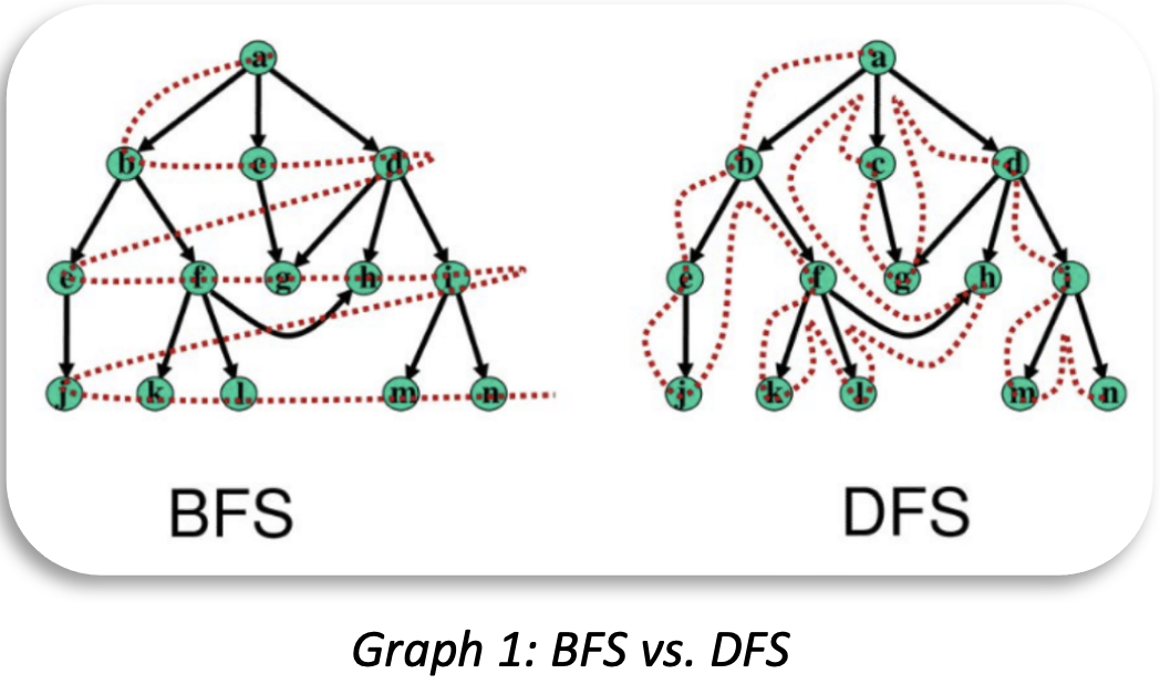
- BFS (Breadth First Search): Shortest Path, K-hop queries are typically implemented using BFS method. It’s worth clarifying that you may use DFS to implement, say, shortest path finding, but in most real-world applications, particularly with large volumes of data, BFS is guaranteed to be more efficient and logically more straightforward than DFS, period.
- DFS (Depth First Search): Queries like circle finding, auto-networking, template-based path queries, random walks desire to be implemented using DFS method. If you find it hard to understand the difference between BFS and DFS, refer to the below diagram and a college textbook on Graph Theory.
- Combination of Both (BFS + DFS): There are scenarios where both BFS and DFS are applied, such as template-based K-hop queries, customized graph algorithms, etc.
Graph 1 illustrates the traversal difference between BFS and DFS. In short, under BFS mode, if qualified 1st hop neighbors are not all visited first, the access to any 2nd hop neighbor will not start, and traversal will continue in this way until all data(neighbors) are visited hop after hop. Based on such excerpt, it’s not hard to tell that if a certain K-hop or shortest-path query only returns a pre-defined limited number of neighbors or paths (say, 1 or 10), it’s guaranteed that the query implementation is wrong! Because you do NOT know the total number of qualified neighbors or paths beforehand.
Typical Benchmark Datasets
There are 3 types of datasets for graph system benchmarking:
- Social or Road Network Dataset: Typical social network datasets like Twitter-2010 and Amazon0601 have been commonly used for graph database benchmarking. There are also road network or web-topology based datasets used in academic benchmarks such as UC Berkeley’s GAP.
- Synthetic Dataset: HPC (High-Performance Computing) organization Graph-500 has published some synthetic datasets for graph system benchmark. International standard organization LDBC (Linked Data Benchmark Council) also use data-generating tools to create synthetic social-network datasets for benchmarking purposes.
- Financial Dataset: The latest addition to the family of graph benchmark datasets is financial dataset, mostly are found in private and business-oriented setup, because the data are often based on real transactions. There are several public datasets such as Alimama’s e-commerce dataset, and LDBC’s FB (FinBench) dataset which is being draft and to be released toward the end of 2022 (to replace the LDBC’s SNB dataset which does NOT reflect real-world financial business challenges in terms of data topology and complexity).
As graph database and computing technologies and products continue to evolve, it’s not hard to see that more graph datasets will emerge and better reflect real-world scenarios and business challenges.
Twitter-2010 (42 Million vertices, 1.47 Billion edges, sized at 25GB, downloadable from http://an.kaist.ac.kr/traces/WWW2010.html) is commonly used in benchmarking, we’ll use it as a level playing field to explain how to interpret a benchmark report and how to validate results in the report.
Before we start, let’s get ourselves familiar with a few concepts in graph data modeling by using the Twitter dataset as an example:
- Directed Graph: Every edge has a unique direction, in Twitter, an edge is composed of a starting vertex and an ending vertex, which map to the 2 IDs separated by TAB on each line of the data file, and the significance of the edge is that it indicates the starting vertex (person) follows the ending vertex (person). When modeling the edge in a graph database, the edge will be constructed twice, the first time as StartingVertex EndingVertex, and the second time as EndingVertex StartinVertex (a.k.a, the inverted edge), this is to allow traversing the edge from either direction. If the inverted edge is not constructed, queries’ results will be inevitably wrong (We’ll show you how later).
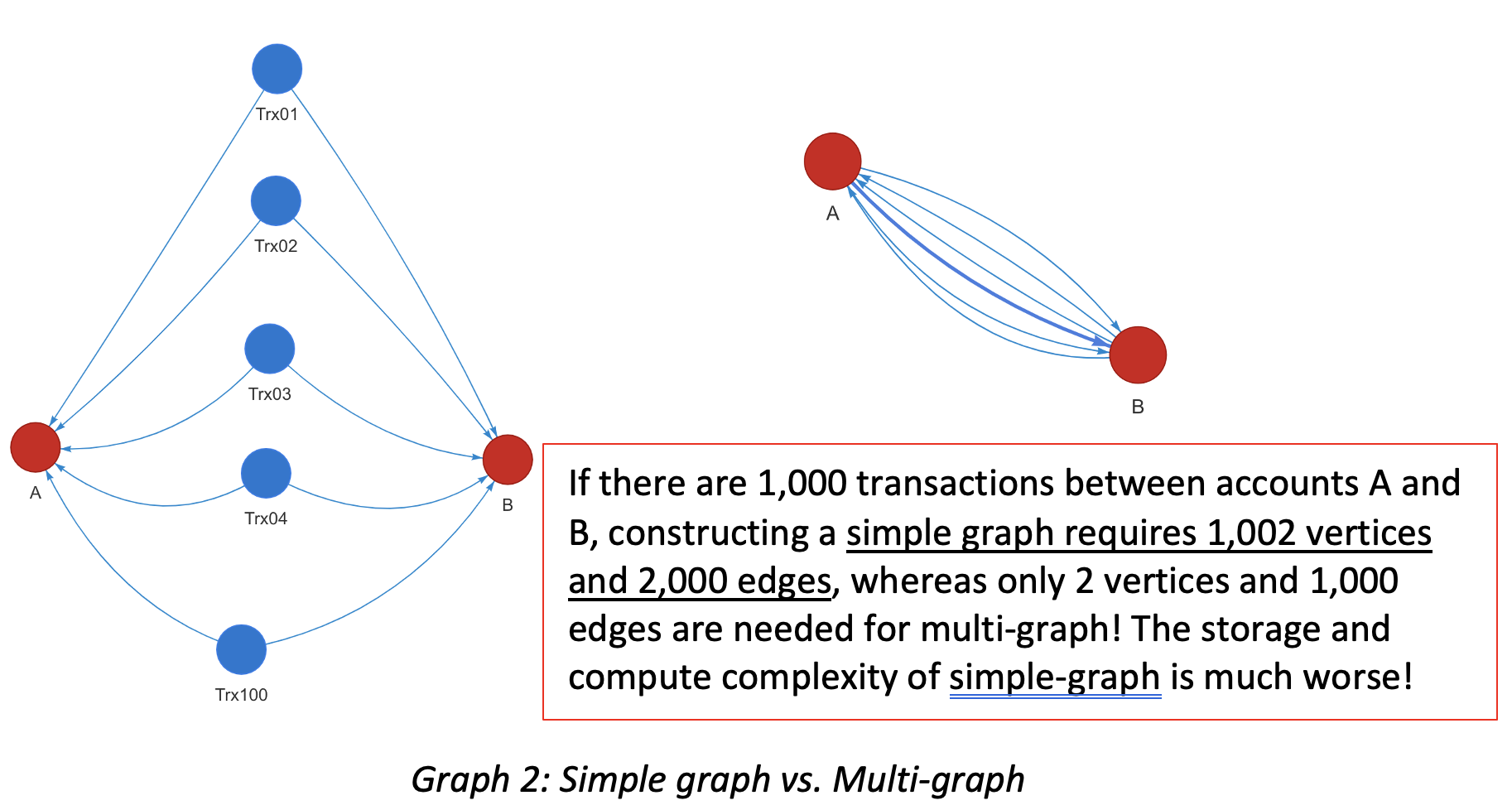
- Simple-graph vs. Multi-graph: If there are more than 2 edges of the same kind between a pair of vertices in either direction, it’s a multi-graph, otherwise, it’s a simple-graph. Twitter and all social network datasets are considered simple graphs because it models a simple following relationship between the users. In financial scenarios, assuming user accounts are vertices and transactions are edges, there could be many transactions in between two accounts, therefore many edges. Some graph databases are designed to be simple-graph instead of multi-graph, this will create lots of problems in terms of data modeling efficiency and query results correctness.
- Node-Edge Attributes:Twitter data does NOT carry any node or edge attribute other than the designated direction of the edge. This is different from transactional graph in financial scenarios, where both node and edge may have many attributes so that filtering, sorting, aggregation, attribution analysis can be done with the help of these attributes. There are so-called graph database systems that do NOT support the filtering by node or edge attributes, which are considered impractical and lack of commercial values.
Report Interpretation
Generally speaking, there are at least 5 parts of a graph database benchmark report:
- Testing Bed/Environment: Software and hardware environment, testing datasets, etc.
- Data Ingestion: Volume data loading, database startup time, etc.
- Query Performance: Queries against meta-data, K-hop, shortest-path, algorithm, etc.
- Real-time Update: Modification to graph data’s topology (meta-data) then query against the updated data to validate results.
- Feature Completeness & Usability: Support of API/SDK for secondary development, GQL, management and monitoring, system maintenance toolkits and disaster recovery, etc.
Most benchmark reports would cover the first 3 parts, but not the 4th or 5th parts – the 4th part reflects if the subject database is more of the OLTP/HTAP type or OLAP focused, with the main difference lying at the capability to process dynamically changing datasets. Clearly, if a graph system claims to be capable of OLTP/HTAP, it must allow data to be updated and queried all the time, instead of functioning as a static data warehouse like Apache Spark, or data projections must be finished first before queries can be run against the just-finished static projection like Neo4j does.
Testing Bed
Almost all graph database products are built on X86 architecture as X86-64 CPU powered servers dominate the server marketplace. The situation has recently changed given the rise of ARM, due to its simplistic RISC (instead of X86’s CISC) therefore greener design. There are growing number of commodity PC servers basing on ARM CPUs nowadays. However, only 2 graph database vendors are known to natively support ARM-64 CPU architecture, they are Ultipa and ArangoDB, while other vendors tend to use virtualization or emulation methods which tend to be dramatically slower than native method.
The core hardware configurations are CPU, DRAM, external storage and network bandwidth. The number of CPU cores are most critical, as more cores mean potentially higher parallelism and better system throughput. Most testing beds settle on 16-core and 256GB configuration, however not all graph systems can leverage multiple cores for accelerated data processing, for instance, even enterprise edition Neo4j leverages up to 4-vCPU in terms of parallelization. If another system can leverage 16-vCPU, the performance gain would be at least 400%.
|
Hardware |
Typical Configuration (For Twitter-2010) |
|
# of Server Instances |
3 Normally in Master-Slave setup |
|
CPU |
Intel Xeon 16-core (32 vCPUs) Alternatively, ARM-64 16-core (32vCPUs) |
|
RAM |
256GB |
|
Hard Disk |
1TB HDD (Cloud Based) or SSD (for better I/O) |
|
Network |
5Gbps |
|
Cloud Service Provider |
Azure, AWS, Google Cloud, Alibaba Cloud, or some private cloud environment |
The table above illustrates typical hardware configuration for graph system benchmarking. It’s worthwhile pointing out that graph database is computing first, unlike RDBMS, Data Warehouse or Data Lake systems which are storage first and compute is 2nd class citizen that’s attached to the storage engine. In another word, traditional DBMS addresses I/O-intensive challenges first, while graph system solves computing-intensive challenges first. While both challenges may intersect with each other, that’s why a performance-oriented graph database should set both computing and storage as its first-class citizens.
The software environment is trivial as all known graph systems settle on Linux OS, and leverage container and virtualization technologies for encapsulation and isolation.
Data Ingestion
Data ingestion has a few indicators to watch out for:
- Dataset volume, topological complexity (or density)
- Ingestion time
- Storage space
Data volume concerns the total number of vertices and edges, plus complexity (or density), which is normally calculated using the following formula (for directed simple graph):
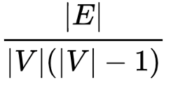
Where |V| annotates the total number of vertices, and |E| for total number of edges. Per this formula, the highest possible density of a smiple graph is 1. However, as we pointed out earlier, most real-world graphs are NOT simple-graph, but multi-graph, meaning multiple edges may exist between any two vertices, therefore it makes more sense to use vertex-to-edge ratio (|E|/|V|) as a “density” indicator. Taking Twitter-2010 as an example, its ratio is 35.25 (while density is 0.000000846). For any graph dataset with a ratio higher than 10, deep traversal against the dataset poses as great challenge due to exponentially complexity, for instance, 1-hop = 10 neighboring vertices, 2-hop = 100 vertices, 3-hop = 1,000 vertices, and 10-hop = 10,000,000,000.
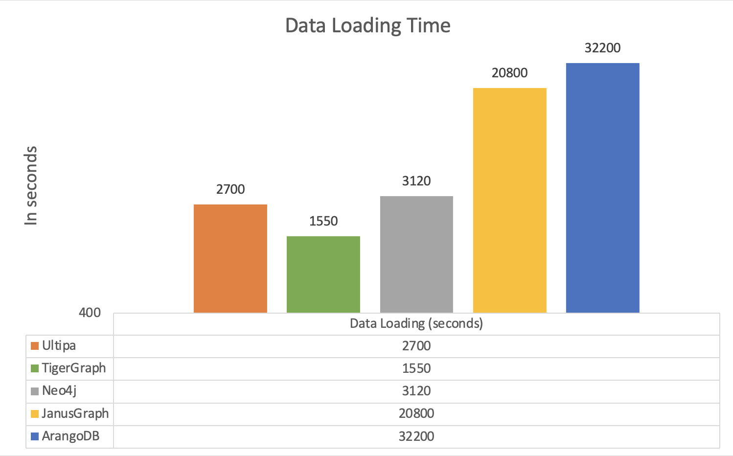
Ingestion time and storage usage show that how soon can a graph database load the entire dataset, and how much storage space it uses on filesystem. Clearly, for loading time, the shorter the better. Storage space is less of a concern nowadays as storage is super cheap, different database systems may have quite different storage mechanism in terms of replication, sharding, partitioning, normalization and other techniques that may affect computing efficiency and high-availability. The table below shows the data ingestion performance of different graph DBMSes.
|
Raw Data |
Twitter-2010, 42M Nodes, 1.47B Edges, 24.6GB in Size | ||||
|
Graph DB |
Ultipa |
TigerGraph |
Neo4j |
JanusGraph |
ArangoDB |
|
Ingestion Time (seconds) |
2700 |
780 |
3120 |
20800 |
32200 |
|
Relative Time |
1 |
2.98 |
6 |
40 |
61.92 |
|
Storage Space |
30GB |
12GB* |
55GB |
56GB |
128GB |
|
Relative Space |
2.5 |
1 |
4.58 |
4.67 |
10.67 |
Note that Tigergraph stores each edge unidirectionally instead of bidirectionally, this alone saves 50% storage space, but it’s incorrect. If Tigergraph were to store properly, it would occupy at least 24GB. If a system only stores an edge unidirectionally, it would generate incorrect results for queries like K-hop, Path or algorithm, and we’ll get to that later.
Query Performance
There are mainly 3 types of graph queries:
- Query for Neighbors:also known as K-hop
- Path: Shortest path queries are commonly used for simplicity (ease-of-comparison)
- Algorithm: Commonly benchmarked algorithms include PageRank, Connected Component, LPA, and Similarity. Some performance-oriented graph databases also benchmark Louvain community detection algorithm which is considered more complex and challenging
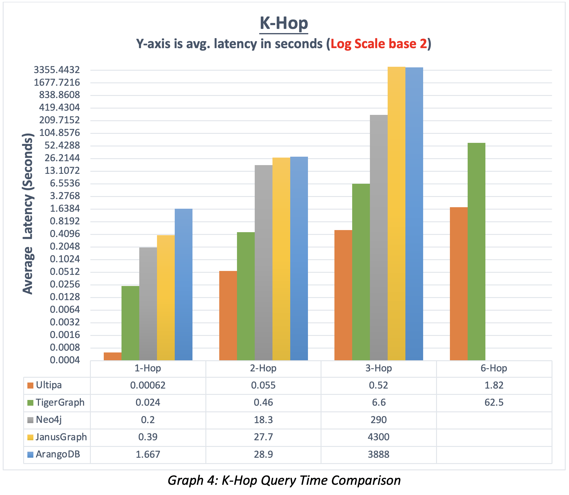
K-Hop measures query latency at different depth. Taking Twitter-2010 as an example, it makes sense to measure the performance of 1-Hop and all the way to 6-Hop. Most databases can handle 1-hop without problem, but 2-hop and beyond are much more challenging, very few systems can return beyond 3-hop. If a system can finish 6-hop (considered deep traversal) within 10 seconds, it’s considered a real-time graph database, because 6-hop traversal of most vertices of Twitter dataset would basically touch base with 95% of all 1.5 billion edges and vertices, which translates to the computing power of traversing over 150 million nodes and edges every second.
For any given dataset and any designated starting vertex, K-hop query result is deterministic, therefore all benchmarking systems should return the exact result. Common mistakes with K-hop are:
- DFS instead of DFS for traversal (wrongful implementation)
- No deduplication (redundant and incorrect results)
- Partial traversal (violation of the definition of K-hop)
|
Dataset |
Twitter-2010 | ||||
|
Graph System |
Ultipa |
TigerGraph |
Neo4j |
JanusGraph |
ArangoDB |
|
1-Hop (second) |
0.00062 |
0.024 |
0.2 |
0.39 |
1.667 |
|
2-Hop (second) |
0.055 |
0.46 |
18.3 |
27.7 |
28.9 |
|
3-Hop (second) |
0.52 |
6.6 |
290 |
4300 |
3888 |
|
6-Hop (second) |
1.82 |
62.5 |
N/A |
N/A |
N/A |
|
23-Hop (second) |
1.92 |
N/A |
N/A |
N/A |
N/A |
Note, Ultipa Graph is the only system that has published its ultra-deep traversal results, vertices having neighbors that are 23-hop away, which reflects the system’s capability to deeply penetrate data in real-time while other systems may take hours or even days to complete, or never finish.
Shortest-Path query is considered a special form of K-hop query, the difference lies at fixing both the starting vertex and ending vertex and find all possible paths in between. Note that in dense dataset like Twitter-2010, there are possibly millions of shortest paths between a pair of vertices. Only 3 graph database vendors have published their benchmark results against Twitter, but Ultipa is the only vendor that has published the exact number of paths as shown in the below table. Some vendors return with only 1 shortest path, which is both ridiculously wrong and problematic. In many real-world scenarios, such as anti-money laundering paths, transactional networks, it’s imperative to locate all shortest paths between two parties as soon as possible.
|
Testing Item |
Item excerpt |
Starting Vertex |
End Vertex |
# of Shortest Paths |
Execution Time |
Average Execution Time |
|
Find All Shortest Paths between Random Pairs of Nodes |
For any pair of nodes, query for all the shortest paths between them, log the execution time and total # of paths. |
50329304 |
21613682 |
25389 |
0.152s |
0.18s |
|
49449489 |
15645246 |
2080710 |
2.484s | |||
|
39687658 |
47978366 |
46 |
0.053s | |||
|
15489748 |
38548456 |
8 |
0.017s | |||
|
17524616 |
29884615 |
5 |
2.22s | |||
|
33033471 |
37029346 |
273 |
0.018 | |||
|
37048837 |
17555248 |
1114 |
0.01s | |||
|
26895497 |
37893465 |
2 |
0.004s | |||
|
26468497 |
37164965 |
6 |
0.002s | |||
|
54151557 |
37190965 |
30837 |
0.05s |
Graph Algorithm reflects a graph DMBS’ computing power in terms of mass data processing. The number of supported graph algorithms and running speed directly tell a system’s capability and feature completeness. Many graph DBMSes are based on some graph computing engine or framework, which can only handle static dataset, once the dataset is modified, a new projection (loading data into DRAM, comparable to ETL) has to be constructed before the graph algorithms can be relaunched. This is the case for Apache Spark GraphX and Neo4j GDS, the ETL process may take a rather long time, which should be included in the algorithm running time.
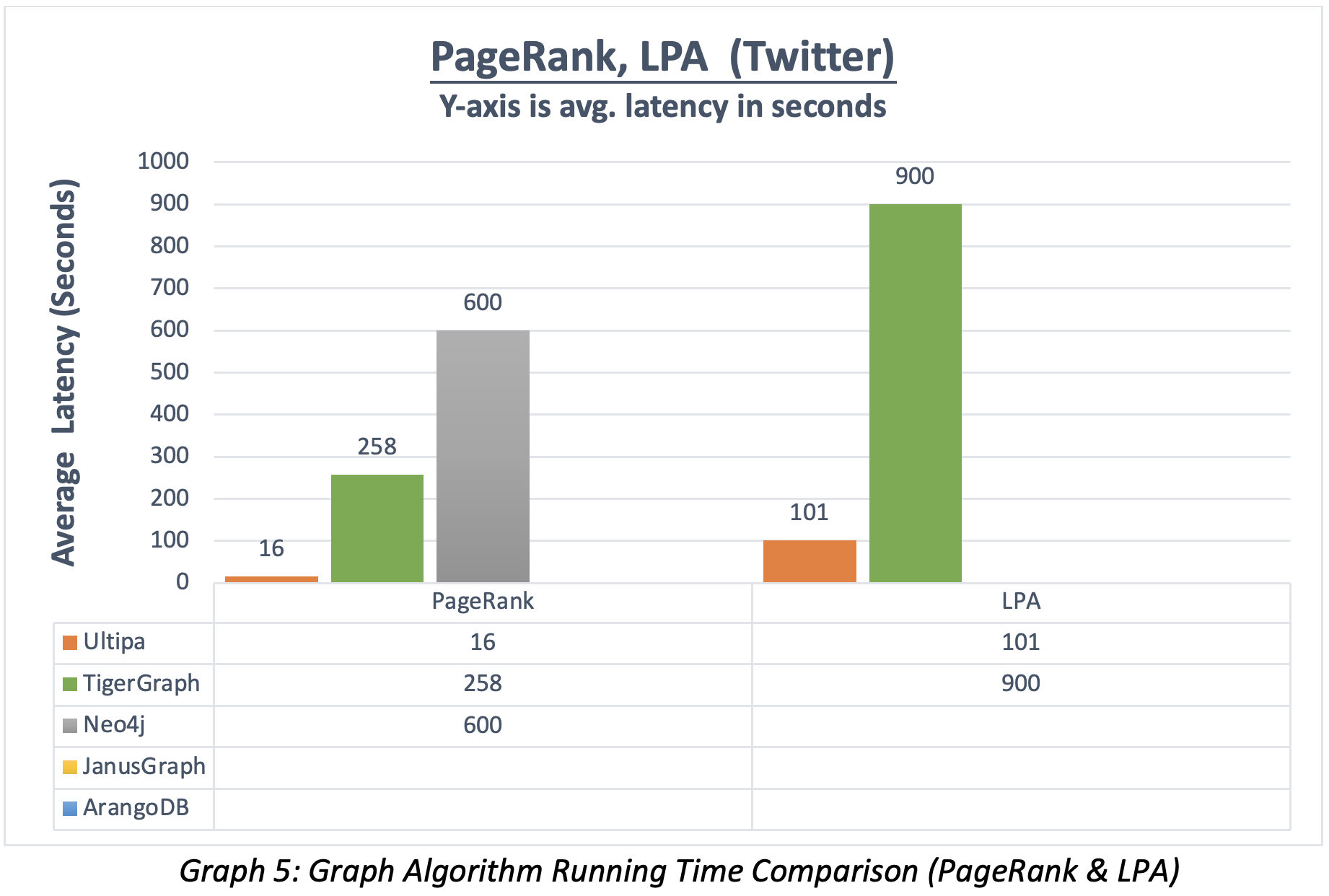
PageRank is the most famous graph algorithm, takes its name from Google co-founder Larry Page. It’s the web search engine’s core ranking algorithm, and one of the 1st algorithm that has been crafted to run parallelly on large-scale distributed systems due to its simple iteration logics and BSP-friendly design. The algorithm running results conveniently tell the ranking (importance) of each vertex (entity) is comparing with the rest of the dataset. For commercial grade implementation, there are also features like database write-back, filesystem write-back, streaming write-back, results ranking, etc.
The 2 essential features of PageRank to watch out for:
- PageRank must run against the entire dataset, not partially
- Results should be fully ranked, and return Top-N as needed
We noticed that some graph DBMS only calculates against a partial dataset, this is a direct violation of the definition of PageRank which is to iterate through entire dataset. Neo4j GDS is a typical example that allows the algorithm to run against, say, 1,000 vertices if the input parameter provided has a limit of 1,000. Taking Twitter-2010 as an example, the result would be 100% wrong, because running against 1,000 vertices is only 0.000025% of the entire dataset. On the other hand, if the results are not ranked, it’s up to the business layer (application layer) to do the ranking which clearly isn’t acceptable. We found that most graph DBMS benchmarking results do not touch base on these issues.
The table below lists the benchmarking logics of PageRank, and list of top-10 returning vertices:
|
Testing Item |
Item excerpt |
Ultipa Testing Results Top-10 Highest Ranked Vertices |
Execution Time (in seconds) |
|
Impact Analysis |
Run PageRank algorithm for 10 iterations, with damping-0.8, return the top-10 highest ranked vertices and their rankings, log the total execution time. |
813286,14276.1 14224719,12240 31567254,10288.6 15131310,9860.32 16049683,8546.38 7040932,6775.97 14075928,6672.9 12687952,5345.58 5380672,5021.32 26784273,2886.91 |
23s |
LPA (Label Propagation Algorithm) is a classic community-detection algorithm, it propagates predefined labels across all vertices iteratively until a stable state is achieved. Comparing to Pagerank, LPA is computationally more complex, and returns total number of communities per vertex-label aggregation. There are also various write-back options to look at when invoking LPA.
Louvain community detection algorithm is computationally more complex than LPA, and iterate through all vertices repeatedly to calculate maximum modularity of the entire dataset. Very few graph DBMS vendors prefer to benchmark Louvain on dataset larger than 100 million nodes and edges. The original Louvain algorithm was implemented using C++ yet in a sequential fashion, on a typical billion-scale dataset, it would require 2.5 hours to finish, if this is to be done in Python, it would last at least a few hundred hours (weeks). Ultipa is the only vendor that has published Louvain’s benchmark results on dataset sized over 1 billion.
|
Dataset |
Twitter-2010: 41.6M, 1470M, 24.6GB | ||||
|
Graph DB |
Ultipa |
TigerGraph |
Neo4j |
JanusGraph |
ArangoDB |
|
PageRank (Seconds) |
23 |
258 |
600 |
N/A Unfinished |
N/A Unfinished |
|
LPA (Seconds) |
80 |
900 |
N/A Unfinished |
N/A Unfinished |
N/A Unfinished |
|
Louvain (Seconds) |
402 |
N/A Not-Tested |
N/A Can’t finish projection in 30-min |
N/A Not-Tested |
N/A Not-Tested |
Real-time Updates
There are 2 types of update operations in graph DBMS:
- Meta-data oriented (TP): The operation only affects meta-data like vertex, edge, or their attribute field(s). From traditional DBMS perspective, this is a typical TP-operation (ACID). In graph DBMS, this also means the topology of the graph changes, such as inserting or deleting a node, an edge, or changing an attribute that may affect query results.
- TP+AP operation: This refers to combo operations, where first a meta-data operation is conducted then an AP type of query is launched. This is common with many real-time BI or decision-making related scenarios, such as online fraud detection, where a new transaction or loan-application shows up, and a series of graph-based network and behavior analysis follow the suite.
It is not uncommon that some graph systems use caching mechanism to pre-calculate and store-aside results which do NOT change accordingly after the data contents are change. To validate if a graph database system has the ability to update data contents and allow for accurate data querying in real-time, we create a new edge connecting the provided starting vertex with one of its 3rd-hop neighboring vertex, and compare the 1-to-3-to-6 Hop results before and after the edge is inserted.
The table below shows how the K-hop results change before and after the edge-insertion event. If a system does NOT have the capacity to handle dynamically changing graph data, the K-hop results will stay put.
|
Testing Item |
Item excerpt |
New-Edge Starting Vertex ID |
New-Edge Ending Vertex ID |
Query Depth |
K-Hop Before Edge Adding |
K-Hop After Edge Adding |
|
Update the dataset, do queries against it twice to compare results |
Add a new edge between the starting vertex to one of its 3rd-hop neighboring vertex, and check its 1-hop,3-hop, 6-hop results before and after the edge-adding event |
20727483 |
28843543 |
1 |
973 |
974 |
|
3 |
27206363 |
27210397 | ||||
|
6 |
10028 |
10027 | ||||
|
50329304 |
21378173 |
1 |
4746 |
4747 | ||
|
3 |
29939223 |
29939314 | ||||
|
6 |
9052 |
9052 | ||||
|
26199460 |
32278263 |
1 |
19954 |
19955 | ||
|
3 |
31324330 |
31324333 | ||||
|
6 |
3022 |
3022 | ||||
|
1177521 |
6676222 |
1 |
4272 |
4273 | ||
|
3 |
17139727 |
17139725 | ||||
|
6 |
3101 |
3101 | ||||
|
27960125 |
48271231 |
1 |
7 |
8 | ||
|
3 |
20280156 |
20283107 | ||||
|
6 |
25838 |
25836 | ||||
|
30440025 |
38232241 |
1 |
3386 |
3387 | ||
|
3 |
23120607 |
23121930 | ||||
|
6 |
5437 |
5431 |
In the 2nd part of this article, we'll introduce mechanism to validate the benchmark results, remember that graph DBMS is white-box and explainable AI, we'll show you how everything can be explained in a white-box fashion in part 2. Stay tuned.