Skip-gram Optimization

Overview

The basic Skip-gram model is almost impractical due to various computational demands.

The sizes of matrices $W$ and $W'$ depend on the vocabulary size (e.g., $V = 10000$ ) and the embedding dimension (e.g., $N = 300$ ), where each matrix often contains millions of weights (e.g., $V \cdot N = 3$ million) each! The neural network of Skip-gram is thus made very large, demanding a vast number of training samples to tune these weights.

Additionaly, during each backpropagation step, updates are applied to all output vectors ( $v_{w}^{'}$ ) for matrix $W'$ , even though most of these vectors are unrelated to both the target word and context words. Given the significant size of $W'$ , this gradient descent process is going to be very slow.

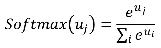
Another substantial cost arises from the Softmax function, which engages all words in the vocabulary to compute the denominator used for normalization.

T. Mikoliv and others introduced optimization techniques in conjunction with the Skip-gram model, including subsampling and negative sampling. These approaches not only accelerate the training process but also improve the quality of embedding vectors.

T. Mikolov, I. Sutskever, K. Chen, G. Corrado, J. Dean, Distributed Representations of Words and Phrases and their Compositionality (2013)
X. Rong, word2vec Parameter Learning Explained (2016)

Subsampling

Common words in corpus like "the", "and", "is" pose some concerns:

They have limited semantic value. E.g., the model benefits more from the co-occurrence of "France" and "Paris" than the frequent co-occurrence of "France" and "the".
There will be excessive training samples containing these words than the needed amount to train the corresponding vectors.

The subsampling approach is used to address this. For each word in the training set, there is a chance to discard it, and less frequent words are discarded less often.

First, calculate the probability of keeping a word by:

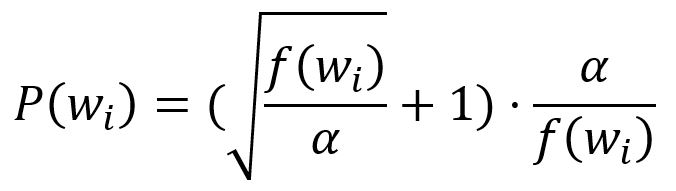
where $f (w_{i})$ is the frequency of the $i$ -th word, $α$ is a factor that influences the distribution and is default to $0.001$ .

Then, a random fraction between $0$ and $1$ is generated. If $P (w_{i})$ is smaller than this number, the word is discarded.

For instance, when $α = 0.001$ , then for $f (w_{i}) \leq 0.0026$ , $P (w_{i}) \geq 1$ , so words with frequency $0.0026$ or less will 100% be kept. For a high word frequency like $f (w_{i}) = 0.03$ , $P (w_{i}) = 0.22$ .

In the case when $α = 0.002$ , then words with frequency $0.0052$ or less will 100% be kept. For the same high word frequency $f (w_{i}) = 0.03$ , $P (w_{i}) = 0.32$ .

Thus, a higher value of $α$ increases the probability that frequent nodes are down-sampled.

For example, if word "a" is discarded and is not added to the training sentence "Graph is a good way to visualize data", the resulting sampling outcomes for this sentence will encompass no samples where "a" serves as either the target word or the context word.

Negative Sampling

In the negative sampling approach, when a positive context word is sampled for a target word, a total of $k$ words are simultaneously chosen as negative samples.

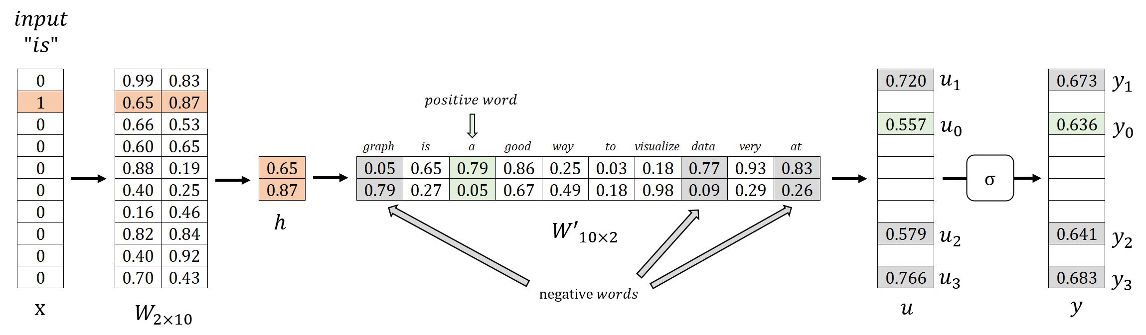
For instance, let's consider the simple corpus when discussing the basic Skip-gram model. This corpus comprises a vocabulary of 10 words: graph, is, a, good, way, to, visualize, data, very, at. When the positive sample (target, content): (is, a) is generated using a sliding window, we select $k = 3$ negative words graph, data and at to accompany it:

Target Word		Context Word	Expected Output
is	Positive Sample	a	1
	Negative Samples	graph	0
		data	0
		at	0

With negative sampling, the training objective of the model shifts from predicting context words for the target word to a binary classification task. In this setup, the output for the positive word is expected as $1$ , while the outputs for the negative words are expected as $0$ ; other words that do not fall into either category are disregarded.

Consequently, during the backpropagation process, the model only updates the output vectors $v_{w}^{'}$ associated with the positive and negative words to improve the model's classification performance.

Consider the scenario where $V = 10000$ and $N = 300$ . When applying negative sampling with the parameter $k = 9$ , only $300 \times 10 = 3000$ individual weights in $W'$ will require updates, which is $0.1%$ of the $3$ million weights to be updated without negative sampling!

NOTE

Our experiments indicate that values of $k$ in the range $5 ~ 20$ are useful for small training datasets, while for large datasets the $k$ can be as small as $2 ~ 5$ . (Mikolov et al.)

A probabilistic distribution $P_{n}$ is needed for selecting negative words. The fundamental principle is to prioritize frequent words in the corpus. However, if the selection is solely based on word frequency, it can lead to an overrepresentation of high-frequency words and a neglect of low-frequency words. To address this imbalance, an empirical distribution is often used that involves raising the word frequency to the power of $\frac{3}{4}$ :

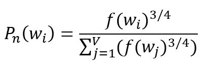
where $f (w_{i})$ is the frequency of the $i$ -th word, the subscript $n$ of $P$ indicates the concept of noise, the distribution $P_{n}$ is also called the noise distribution.

In extreme cases where the corpus contains just two words, with frequencies of $0.9$ and $0.1$ respectively, utilizing the above formula would yield adjusted probabilities of $0.84$ and $0.16$ . This adjustment goes some way in alleviating the inherent selection bias stemming from frequency differences.

Dealing with large corpus can pose challenges in terms of computational efficiency for negative sampling. Therefore, we further adopt a resolution parameter to rescale the noise distribution. A higher value of resolution will provide a closer approximation to the original noise distribution.

Optimized Model Training

Forward Propagation

We will demonstrate with target word is, positive word a, and negative words graph, data and at:

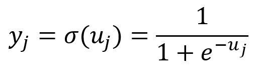
With negative sampling, the Skip-gram model uses the following variation of the Softmax function, which is actually the Sigmoid function ( $σ$ ) of $u_{j}$ . This function maps all components of $u$ within the range of $0$ and $1$ :

Backpropagation

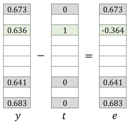
As explained, the output for the positive word, denoted as $y_{0}$ , is expected to be $1$ ; while the $k$ outputs corresponding to the negative words, denoted as $y_{i}$ , are expected to be $0$ . Therefore, the objective of the model's training is to maximize both $y_{0}$ and $1 - y_{i}$ , which can be equivalently interpreted as maximizing their product:

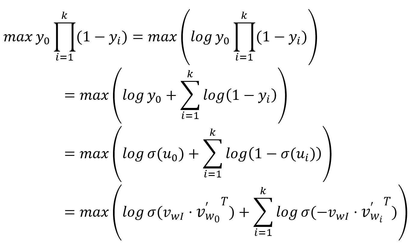
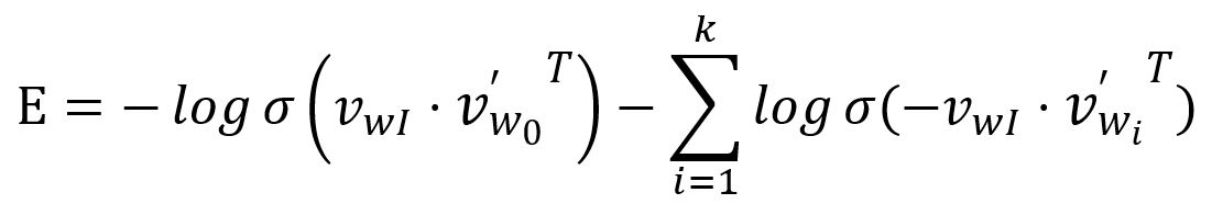
The loss funtion $E$ is then obtained by transforming the above as a minimization problem:

Take the partial derivative of $E$ with respect to $u_{0}$ and $u_{i}$ :

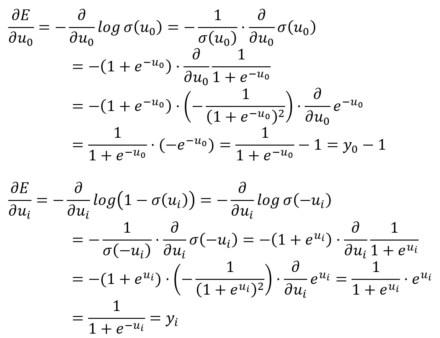
$\frac{\partial E}{\partial u_{0}}$ and $\frac{\partial E}{\partial u_{i}}$ hold a similar meaning to $\frac{\partial E}{\partial u_{j}}$ in the original Skip-gram model, which can be understood as subtracting the expected vector from the output vector:

The process of updating weights in matrices $W'$ and $W$ is straightforward. You may refer to the original form of Skip-gram. However, only weights $w_{11}^{'}$ , $w_{21}^{'}$ , $w_{13}^{'}$ , $w_{23}^{'}$ , $w_{18}^{'}$ , $w_{28}^{'}$ , $w_{1, 10}^{'}$ and $w_{2, 10}^{'}$ in $W'$ and weights $w_{21}$ and $w_{21}$ in $W$ are updated.