Minimum Spanning Tree
✓ File Writeback ✕ Property Writeback ✓ Direct Return ✓ Stream Return ✕ Stats
Overview
The Minimum Spanning Tree (MST) algorithm computes the spanning tree with the minimum sum of edge weights for each connected component in a graph.
The MST has various applications, such as network design, clustering, and optimization problems where minimizing the total cost or weight is important.
Concepts
Spanning Tree
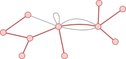
A spanning tree is a connected subgraph that all nodes of a connected graph G= = (V, E) (or a connected component) and forms a tree (i.e., no circles). There may exist multiple spanning trees for a graph, and each spanning tree must have (|V| - 1) edges.
The 11 nodes in the graph below, along with the 10 edges highlighted in red, form a spanning tree of this graph:
Minimum Spanning Tree (MST)
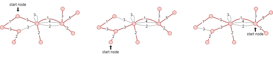
The MST is the spanning tree that has the minimum sum of edge weights. The construction of the MST starts from a given start node. The choice of the start node does not impact the correctness of the MST algorithm, but it can affect the structure of the MST and the order in which edges are added. Different start nodes may result in different MSTs, but all of them will be valid MSTs for the given graph.
After assigning edge weights to the above example, the three possible MSTs with different start nodes are highlighted in red below:
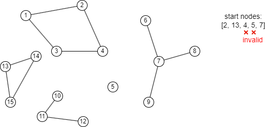
Regarding the selection of start nodes:
- Each connected component requires only one start node. If multiple start nodes are specified, the first one will be considered valid.
- No MST will be computed for connected components that do not have a specified start node.
- Isolated nodes are not considered valid start nodes for computing the MST.
Considerations
- The MST algorithm ignores the direction of edges but calculates them as undirected edges.
Syntax
- Command:
algo(mst) - Parameters:
Name | Type | Spec | Default | Optional | Description |
|---|---|---|---|---|---|
| ids / uuids | []_id / []_uuid | / | / | Yes | ID/UUID of the start nodes; the system chooses the start node for each connected component if not set |
| edge_schema_property | []@<schema>?.<property> | Numeric type, must LTE | / | No | Edge properties to use as weights; for each edge, the specified property with the smallest value is considered as its weight; edges without any specified property will not be included in any MST |
| limit | int | ≥-1 | -1 | Yes | Number of results to return, -1 to return all results |
Examples
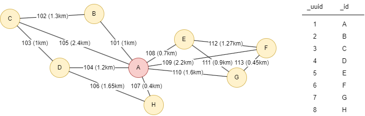
The example graph is as below, node A is an electric center, node B~H are the surrounding villages. Each edge is labeled with its UUID and the distance between the connected locations, which represents the required cable length:
File Writeback
Spec | Content | Description |
|---|---|---|
| filename | _id--[_uuid]--_id | One-step path in the MST: (start node)--(edge)--(end node) |
UQLalgo(mst).params({
  uuids: [1],
  edge_schema_property: 'distance'
}).write({
  file:{
    filename: 'solution'
    }
})
Results: File solution
FileA--[107]--H
A--[108]--E
E--[111]--G
F--[113]--G
A--[101]--B
A--[104]--D
C--[103]--D
Direct Return
Alias Ordinal | Type | Description |
|---|---|---|
| 0 | []path | One-step path in the MST: _uuid (start node) -- [_uuid] (edge) -- _uuid (end node) |
UQLalgo(mst).params({
  ids: 'A',
  edge_schema_property: '@connect.distance'
}) as mst
return mst
Results: mst
| 1--[107]--8 |
| 1--[108]--5 |
| 5--[111]--7 |
| 6--[113]--7 |
| 1--[101]--2 |
| 1--[104]--4 |
| 3--[103]--4 |
Stream Return
Alias Ordinal | Type | Description |
|---|---|---|
| 0 | []path | One-step path in the MST: _uuid (start node) -- [_uuid] (edge) -- _uuid (end node) |
UQLalgo(mst).params({
  uuids: [1],
  edge_schema_property: 'distance'
}).stream() as mst
with pedges(mst) as mstUUID
find().edges(mstUUID) as edges
return sum(edges.distance)
Results: 5.65