Skip-gram

The Skip-gram (SG) model is a prominent approach designed for creating word embeddings in the field of natural language processing (NLP). It has also been used in graph embedding algorithms such as Node2Vec and Struc2Vec to generate node embeddings.

Background

The origin of the Skip-gram model can be traced back to the Word2Vec algorithm. Word2Vec maps words to a vector space, where semantically similar words are represented by vectors that are close in proximity. Google's T. Mikolov et al. introduced Word2Vec in 2013.

• T. Mikolov, K. Chen, G. Corrado, J. Dean, Efficient Estimation of Word Representations in Vector Space (2013)
• X. Rong, word2vec Parameter Learning Explained (2016)

In the realm of graph embedding, the inception of DeepWalk in 2014 marked the application of the Skip-gram model to generate vector representations of nodes within graphs. The core concept is treating nodes as "words", the node sequences generated by random walks as "sentences" and "corpus".

• B. Perozzi, R. Al-Rfou, S. Skiena, DeepWalk: Online Learning of Social Representations (2014)

Subsequent graph embedding methods such as Node2Vec and Struc2Vec have enhanced the DeepWalk approach while still leveraging the Skip-gram framework.

We will illustrate the Skip-gram model using the context of its original application in natural language processing.

Model Overview

The fundamental principle underlying Skip-gram is to predict a set of context words for a given target word. As depicted in the diagram below, the input word, denoted as $w(t)$, is fed into the model; the model then generates four context words related to $w(t)$: $w(t-2)$, $w(t-1)$, $w(t+1)$, and $w(t+2)$. Here, the symbols $+$/$-$ signify the preceding and succeeding context in relation to the target word. The number of context words produced can be adjusted as needed.

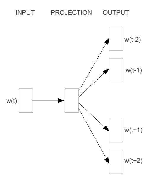
However, it's important to recognize that the ultimate objective of the Skip-gram model is not prediction. Instead, its real task to derive the weight matrix found within the mapping relationship (indicated as PROJECTION in the diagram), which effectively represents the vectorized representations of words.

Corpus

A corpus is a collection of sentences or texts that a model utilizes to learn the semantic relationships between words.

Consider a vocabulary containing 10 distinct words drawn from a corpus: graph, is, a, good, way, to, visualize, data, very, at.

These words can be constructed into sentences such as:

Graph is a good way to visualize data.

Sliding Window Sampling

The Skip-gram model employs the sliding window sampling technique to generate training samples. This method uses a "window" that moves sequentially through each word in the sentence. The target word is combined with every context word before and after it, within a certain range window_size.

Below is an illustration of the sampling process when window_size$=1$.

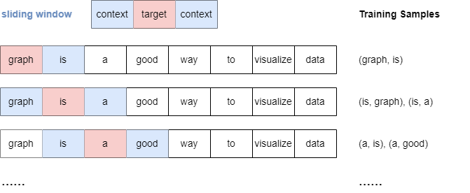
It's important to note that when window_size$>1$, all context words falling within the specified window are treated equally, regardless of their distance from the target word.

One-hot Encoding

Since words are not directly interpretable by models, they must be converted into machine-understandable representations.

One common method for encoding words is the one-hot encoding. In this approach, each word is represented as a unique binary vector where only one element is "hot" ($1$) while all others are "cold" ($0$). The position of the $1$ in the vector corresponds to the index of the word in the vocabulary.

Here is how one-hot encoding is applied to our vocabulary:

Skip-gram Architecture

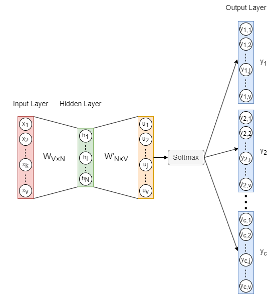
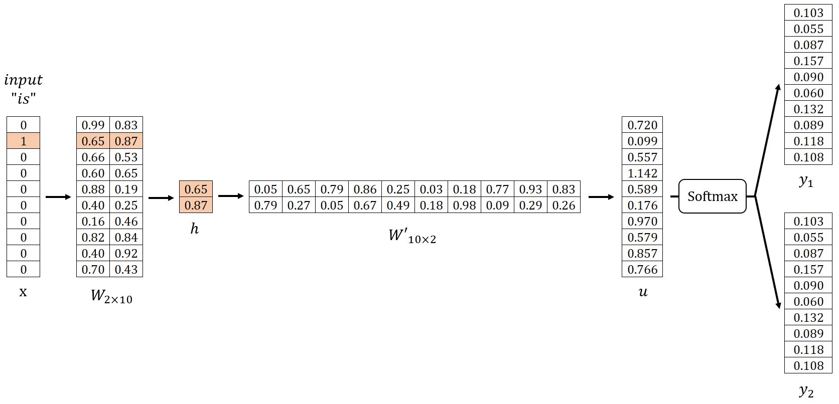
The architecture of the Skip-gram model is depicted as above, where:

• The input vector $x_{V\times 1}$ is the one-hot encoding of the target word, and $V$ is the number of words in the vocabulary.
• $W_{V\times N}$ is the input→hidden weight matrix, and $N$ is the dimension of word embeddings.
• $h_{N\times 1}$ is the hidden layer vector.
• ${W\prime }_{N\times V}$ is the hidden→output weight matrix. $W\prime$ and $W$ are different, $W\prime$ is not the transpose of $W$.
• $u_{V\times 1}$ is the vector before applying the activation function Softmax.
• The output vectors $y_c$ ($c=1\mathrm{, }2\mathrm{, }\mathrm{...}\mathrm{, }C$) are also referred to as panels, $C$ panels correspond to $C$ context words of the target word.

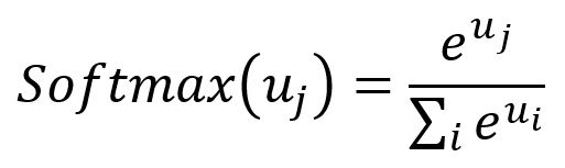
Softmax: Softmax function as an activation function, serving to normalize a numerical vector into a probability distribution vector. In this transformed vector, the summation of all probabilities equals $1$. The formula for Softmax is as follows:

Forward Propagation

In our example, $V=10$, and set $N=2$. Let's begin by randomly initializing the weight matrices $W$ and $W\prime$ as shown below. We will then use the sample (is, graph), (is, a) for demonstration.

Input Layer → Hidden Layer

Get the hidden layer vector $h$ by:

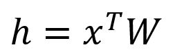
Given $x$ is a one-hot encoded vector with only $x_k=1$, $h$ corresponds to the $k$-th row of matrix $W$. This operation is essentially a simple lookup process:

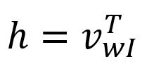
where $v_{wI}$ is the input vector of the target word.

In fact, each row of matrix $W$, denoted as $v_w$, is viewed as the final embedding of each word in the vocabulary.

Hidden Layer → Output Layer

Get the vector $u$ by:

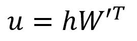
The $j$-th component of vector $u$ equals to the dot product of vector $h$ and the transpose of the $j$-th column vector of matrix $W\prime$:

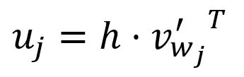
where $v_{w_j}^{\prime }$ is the output vector of the $j$-th word in the vocabulary.

NOTE

In the design of the Skip-gram model, each word within the vocabulary has two distinct representations: the input vector $v_w$ and the output vector $v_w^{\prime }$. The input vector serves as the representation when the word is used as the target, while the output vector represents the word when it acts as the context.

During computation, $u_j$ is essentially the dot product of the input vector of the target word $v_{wI}$ and the output vector of the $j$-th word $v_{w_j}^{\prime }$. The Skip-gram model is also designed with the principle that greater similarity between two vectors yields a larger dot product of those vectors.

Besides, it is important to highlight that only the input vectors are ultimately utilized as the word embeddings. This separation of input and output vectors simplifies the computation process, enhancing both efficiency and accuracy in the model's training and inference.

Get each output panel $y_c$ by:

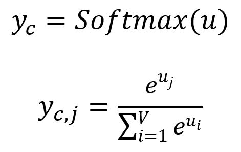
where $y_{c,j}$ is the $j$-th component of $y_c$, representing the probability of the $j$-th word within the vocabulary being predicted while considering the given target word. Apparently, the sum of all probabilities is $1$.

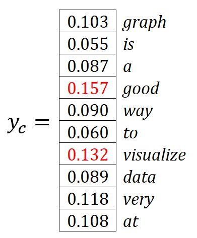
The $\mathrm{C}$ words with the highest probabilities are considered as the predicted context words. In our example, $\mathrm{C}=2$ and the predicted context words are good and visualize.

Backpropagation

To adjust the weights in $W$ and $W\prime$, SGD is used to backpropagate the errors.

Loss Function

We want to maximize the probabilities of the $\mathrm{C}$ context words, i.e., to maximize the product of these probabilities:

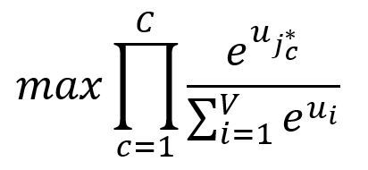
where $j_c^{*}$ is the index of the expected $c$-th output context word.

Since minimization is often considered more straightforward and practical than maximization, we perform some transformations to the above goal:

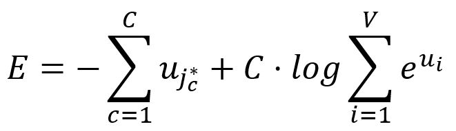
Therefore, the loss function $\mathrm{E}$ of Skip-gram is expressed as:

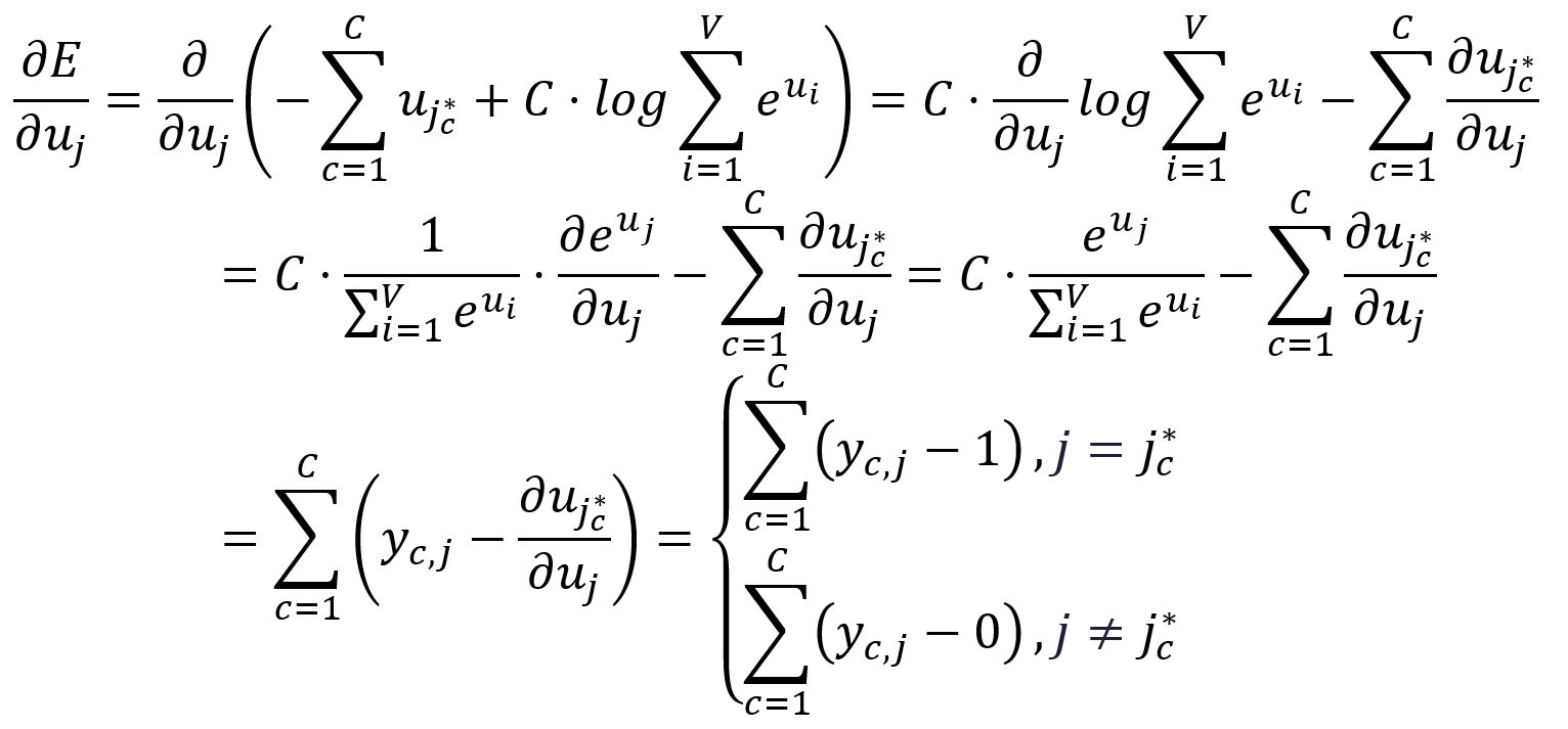
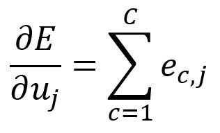
Take the partial derivative of $\mathrm{E}$ with respect to $u_j$:

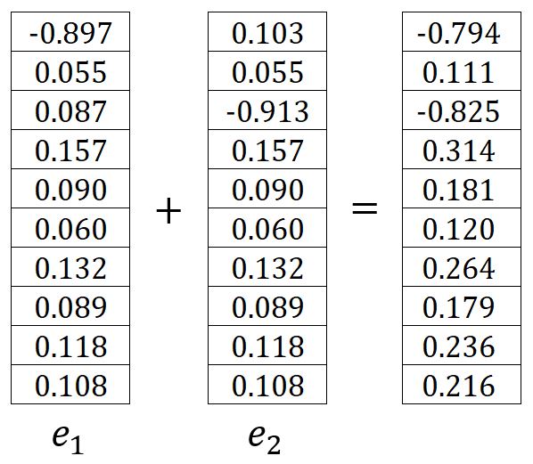
To simply the notaion going forward, define the following:

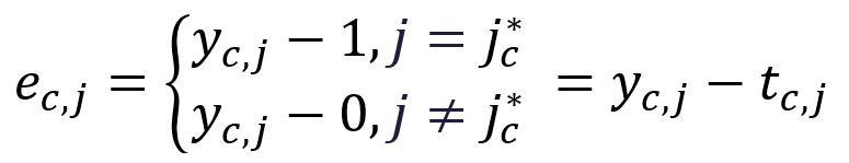
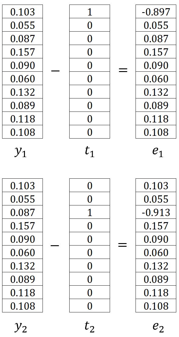
where $t_c$ is the one-hot encoding vector of the $c$-th expected output context word. In our example, $t_1$ and $t_2$ are the one-hot encoded vectors of words graph and a, thus $e_1$ and $e_2$ are calculated as:

Therefore, $\frac{\partial E}{\partial u_j}$ can be written as:

In our example, it is calculated as:

Output Layer → Hidden Layer

Adjustments are made to all weights in matrix $W\prime$, which means that all the output vectors of words are updated.

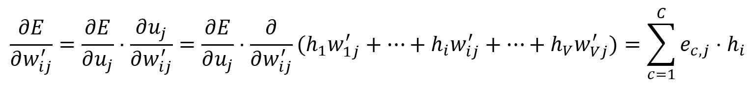
Calculate the partial derivative of $E$ with respect to $w_{ij}^{\prime }$:

Adjust $w_{ij}^{\prime }$ according to the learning rate $\eta$:

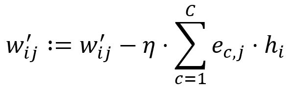
Set $\eta =0.4$. For instance, $w_{14}^{\prime }=0.86$ and $w_{24}^{\prime }=0.67$ are updated to:

$w_{14}^{\prime }=w_{14}^{\prime }-\eta \cdot (e_{1,4}+e_{2,4})\cdot h_1=0.86-0.4\times 0.314\times 0.65=0.78$
$w_{24}^{\prime }=w_{24}^{\prime }-\eta \cdot (e_{1,4}+e_{2,4})\cdot h_2=0.67-0.4\times 0.314\times 0.87=0.56$

Hidden Layer → Input Layer

Adjustments are made only to the weights in matrix $W$ that correspond to the input vector of the target word.

The vector $h$ is obtained by only looking up the $k$-th row of matrix $W$ (given that $x_k=1$):

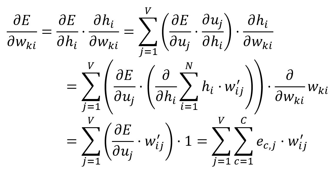
Calculate the partial derivative of $E$ with respect to $w_{ki}$:

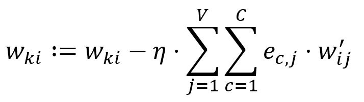
Adjust $w_{ki}$ according to the learning rate $\eta$:

In our example, $k=2$, hence, $w_{21}=0.65$ and $w_{22}=0.87$ are updated:

$\frac{\partial E}{\partial w_{21}}=(e_{1,1}+e_{2,1})\cdot w_{11}^{\prime }+(e_{1,2}+e_{2,2})\cdot w_{12}^{\prime }+\mathrm{...}+(e_{1,10}+e_{2,10})\cdot w_{\mathrm{1,10}}^{\prime }=0.283$
$w_{21}=w_{21}-\eta \cdot \frac{\partial E}{\partial w_{21}}=0.65\mathrm{-}0.4\times 0.283=0.54$

$\frac{\partial E}{\partial w_{22}}=(e_{1,1}+e_{2,1})\cdot w_{21}^{\prime }+(e_{1,2}+e_{2,2})\cdot w_{22}^{\prime }+\mathrm{...}+(e_{1,10}+e_{2,10})\cdot w_{\mathrm{2,10}}^{\prime }=0.081$
$w_{22}=w_{22}-\eta \cdot \frac{\partial E}{\partial w_{22}}=0.87\mathrm{-}0.4\times 0.081=0.84$

Optimization

We have explored the fundamentals of the Skip-gram model. Nevertheless, incorporating optimizations is imperative to ensure the model's computational complexity remains viable and pragmatic for real-world applications. Click here to continue reading.