Gradient descent stands as a foundational optimization algorithm extensively employed in graph embeddings. Its primary purpose is to iteratively adjust the parameters of a graph embedding model to minimize a predefined loss/cost function.

Several variations of gradient descent have emerged, each designed to address specific challenges associated with large-scale graph embedding tasks. Noteworthy variations include Stochastic Gradient Descent (SGD) and Mini-Batch Gradient Descent (MBGD). These variations update model parameters by leveraging the gradient computed from either a single or a smaller subset of data during each iteration.

Basic Form

Consider a real-life scenario: imagine standing atop a mountain and desiring to descend as swiftly as possible. Naturally, there exists an optimal path downwards, yet identifying this precise route is often an arduous undertaking. More frequently, a step-by-step approach is taken. In essence, with each stride to a new position, the next course of action is determined by calculating the direction (i.e., gradient descent) that allows the steepest descent, enabling movement towards the subsequent point in that direction. This iterative process persists until the foot of the mountain is reached.

Revolving around this concept, gradient descent serves as the technique to pinpoint the minimum value along the gradient's descent. Conversely, if the aim is to locate the maximum value while ascending along the gradient's direction, the approach becomes gradient ascent.

Given a function $J(\theta )$, the basic form of gradient descent is:

where $\nabla J$ is the gradient of the function at the position of $\theta$, $\eta$ is the learning rate. Since gradient is the steepest ascent direction, a minus symbol is used before $\eta \nabla J$ to get the steepest descent.

Learning rate determines the length of each step along the gradient descent direction towards the target. In the example above, the learning rate can be thought of as the distance covered in each step we take.

The learning rate typically remains constant during the model's training process. However, variations and adaptations of the model might incorporate learning rate scheduling, where the learning rate could potentially be adjusted over the course of training, decreasing gradually or according to predefined schedules. These adjustments are designed to enhance convergence and optimization efficiency.

Example: Single-Variable Function

For function $J={\theta }^2+10$, its gradient (in this case, same as the derivative) is $\nabla J=J\prime (\theta )=2\theta$.

If starts at position ${\theta }_0=1$, and set $\eta =0.2$, the next movements following gradient descent would be:

• ${\theta }_1={\theta }_0-\eta \times 2{\theta }_0=1-0.2\times 2\times 1=0.6$
• ${\theta }_2={\theta }_1-\eta \times 2{\theta }_1=0.6-0.2\times 2\times 0.6=0.36$
• ${\theta }_3={\theta }_2-\eta \times 2{\theta }_2=0.36-0.2\times 2\times 0.36=0.216$
• ...
• ${\theta }_{18}=0.00010156$
• ...

As the number of steps increases, we progressively converge towards the position $\theta =0$, ultimately reaching the minimum value of the function.

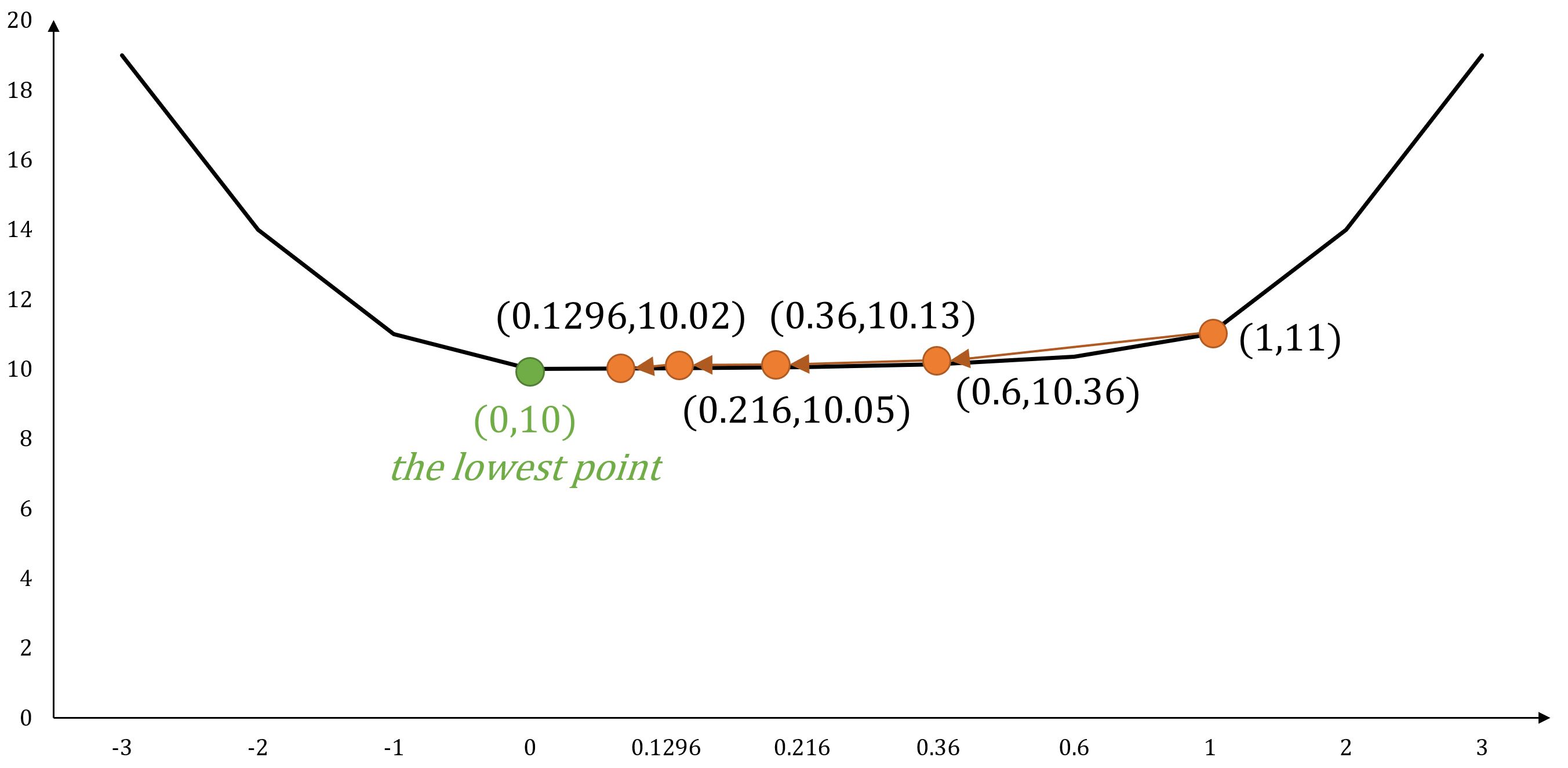
Example: Multi-Variable Function

For function $J(\Theta )={\theta }_1^2+{\theta }_2^2$, its gradient is $\nabla J=(2{\theta }_1\mathrm{, }2{\theta }_2)$.

If starts at position ${\Theta }_0=(-1\mathrm{, }-2)$, and set $\eta =0.1$, the next movements following gradient descent would be:

• ${\Theta }_1=(-1-0.1\times 2\times -1\mathrm{, }-2-0.1\times 2\times -2)=(-0.8\mathrm{, }-1.6)$
• ${\Theta }_2=(-0.64\mathrm{, }-1.28)$
• ${\Theta }_3=(-0.512\mathrm{, }-1.024)$
• ...
• ${\Theta }_{20}=(-0.011529215\mathrm{, }-0.002305843)$
• ...

As the number of steps increases, we progressively converge towards the position $\Theta =(0\mathrm{, }0)$, ultimately reaching the minimum value of the function.

Application in Graph Embeddings

In the process of training a neural network model in graph embeddings, a loss or cost function, denoted as $J(\Theta )$, is frequently employed to assess the disparity between the model's output and the expected outcome. The technique of gradient descent is then applied to minimize this loss function. This involves iteratively adjusting the model's parameters in the opposite direction of the gradient $\nabla J$ until convergence, thereby optimizing the model.

To strike a balance between computational efficiency and accuracy, several variants of gradient descent have been employed in practice, including:

1. Stochastic Gradient Descent (SGD)
2. Mini-Batch Gradient Descent (MBGD)

Example

Consider a scenario where we are utilizing a set of $m$ samples to train a neural network model. Each sample consists of input values and their corresponding expected outputs. Let's use $x^{(i)}$ and $y^{(i)}$ ($i=1\mathrm{, }2\mathrm{, }\mathrm{...}\mathrm{, }m$) denote the $i$-th input value and the expected output.

The hypothesis $h(\Theta )$ of the model is defined as:

Here, $\Theta$ represents the model's parameters ${\theta }_0$ ~ ${\theta }_n$, and $x^{(i)}$ is the $i$-th input vector, consisting of $n$ features. The model uses function $h(\Theta )$ to compute the output by performing a weighted combination of the input features.

The objective of model training is to identify the optimal values of ${\theta }_{\mathrm{j}}$ that lead to the outputs being as close as possible to the expected values. During the start of training, ${\theta }_{\mathrm{j}}$ is assigned random values.

During each iteration of model training, once the outputs for all samples have been computed, the mean square error (MSE) is used as the loss/cost function $J(\Theta )$ to measure the average error between each computed output and its corresponding expected value:

In the standard MSE formula, the denominator is usually $\frac{1}{m}$. However, $\frac{1}{2m}$ is often used instead to offset the squared term when the loss function is derived, leading to the elimination of the constant coefficient for the sake of simplifying subsequent calculations. This modification does not affect the final results.

Subsequently, the gradient descent is employed to update the parameters ${\theta }_j$. The partial derivative with respect to ${\theta }_j$ is calculated as follows:

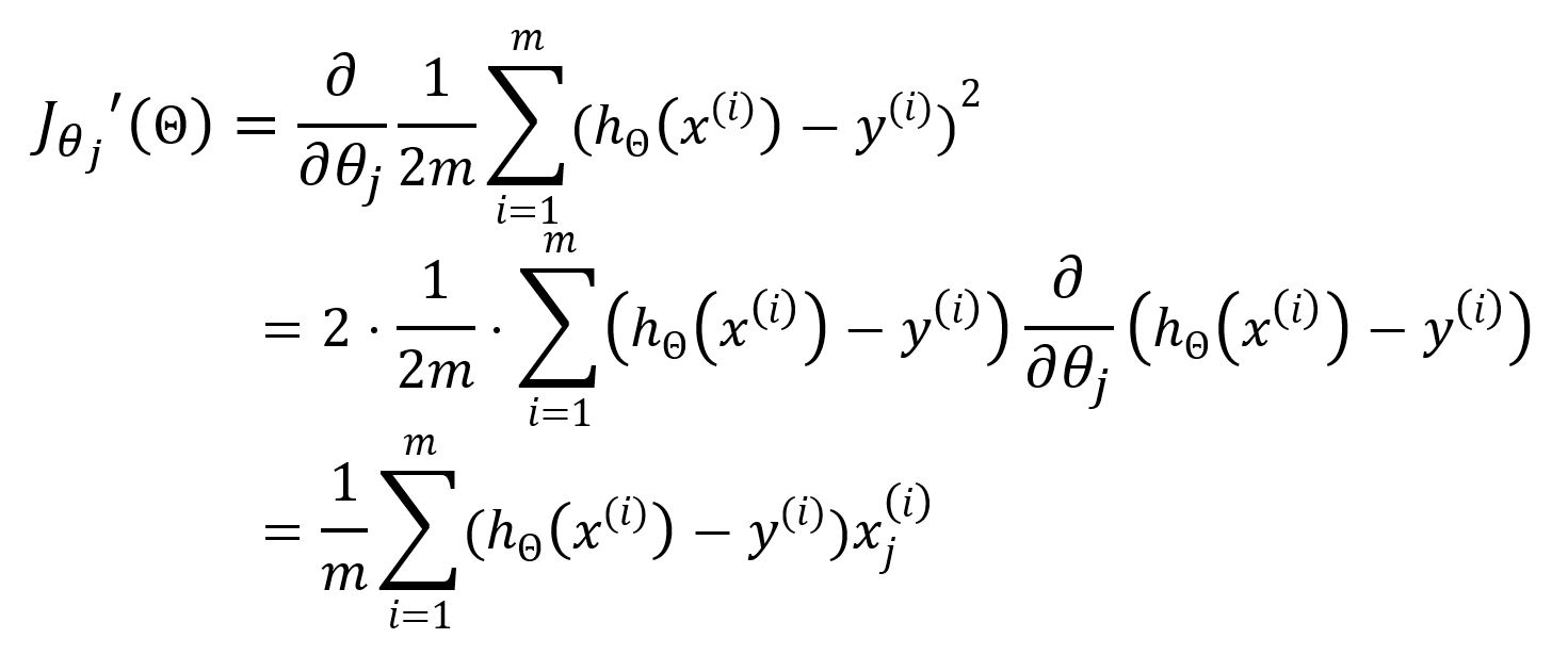
Hence, update ${\theta }_j$ as:

The summation from $i=1$ to $m$ indicates that all $m$ samples are utilized in each iteration to update the parameters. This approach is known as Batch Gradient Descent (BGD), which is the original and most straightforward form of the Gradient Descent optimization. In BGD, the entire sample dataset is used to compute the gradient of the cost function during each iteration.

While BGD can ensure precise convergence to the minimum of the cost function, it can be computationally intensive for large datasets. As a solution, SGD and MBGD were developed to address efficiency and convergence speed. These variations use subsets of the data in each iteration, making the optimization process faster while still seeking to find the optimal parameters.

Stochastic Gradient Descent

Stochastic gradient descent (SGD) only selects one sample in random to calculate the gradient for each iteration.

When employing SGD, the above loss function should be expressed as:

The partial derivative with respect to ${\theta }_j$ is:

Update ${\theta }_j$ as:

The computational complexity is reduced in SGD since it involves the use of only one sample, thereby bypassing the need for summation and averaging. While this enhances computation speed, it comes at the expense of some degree of accuracy.

Mini-Batch Gradient Descent

BGD and SGD both represent extremes - one involving all samples and the other only a single sample. Mini-batch Gradient Descent (MBGD) strikes a balance by randomly selecting a subset of $x\in (1\mathrm{, }m)$ samples for computation.

Mathematical Basics

Derivative

The derivative of a single-variable function $f(x)$ is often denoted as $f\prime (x)$ or $\frac{df}{dx}$, it represents how $f(x)$ changes with respect to a slight change in $x$ at a given point.

Graphically, $f\prime (x)$ corresponds to the slope of the tangent line to the function's curve. The derivative at point $x$ is:

For example, $f(x)=x^2+10$, at point $x=-7$:

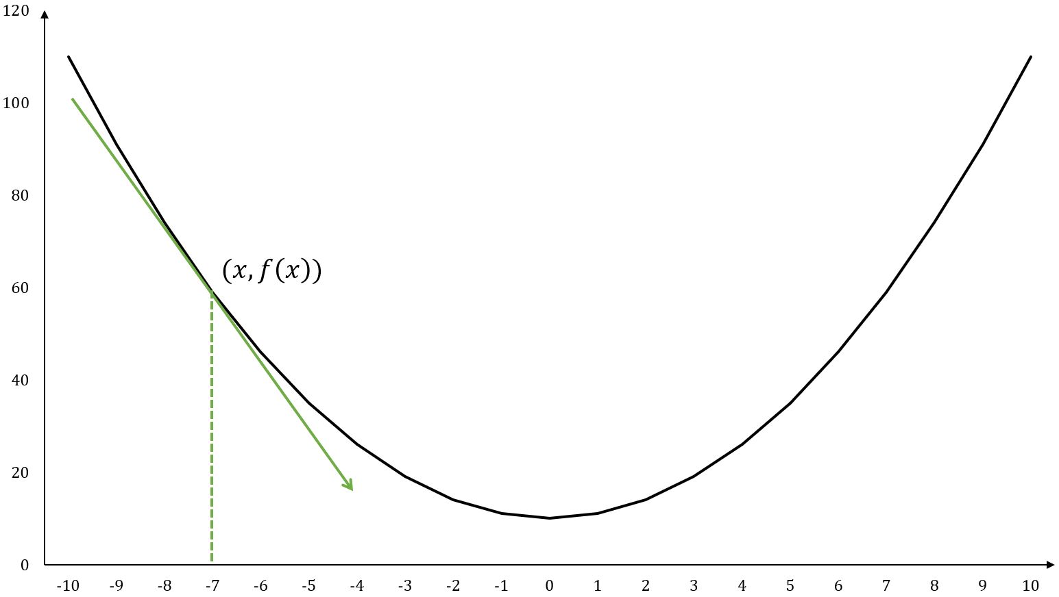
The tangent line is a straight line that just touches the function curve at a specific point and shares the same direction as the curve does at that point.

Partial Derivative

The partial derivative of a multiple-variable function measures how the function changes when one specific variable is varied while keeping all other variables constant. For a function $f(x,y)$, its partial derivative with respect to $x$ at a particular point $(x,y)$ is denoted as $\frac{\partial f}{\partial x}$ or $f_x^{\prime }$:

For example, $f(x,y)=x^2+y^2$, at point $x=-4$, $y=-6$:

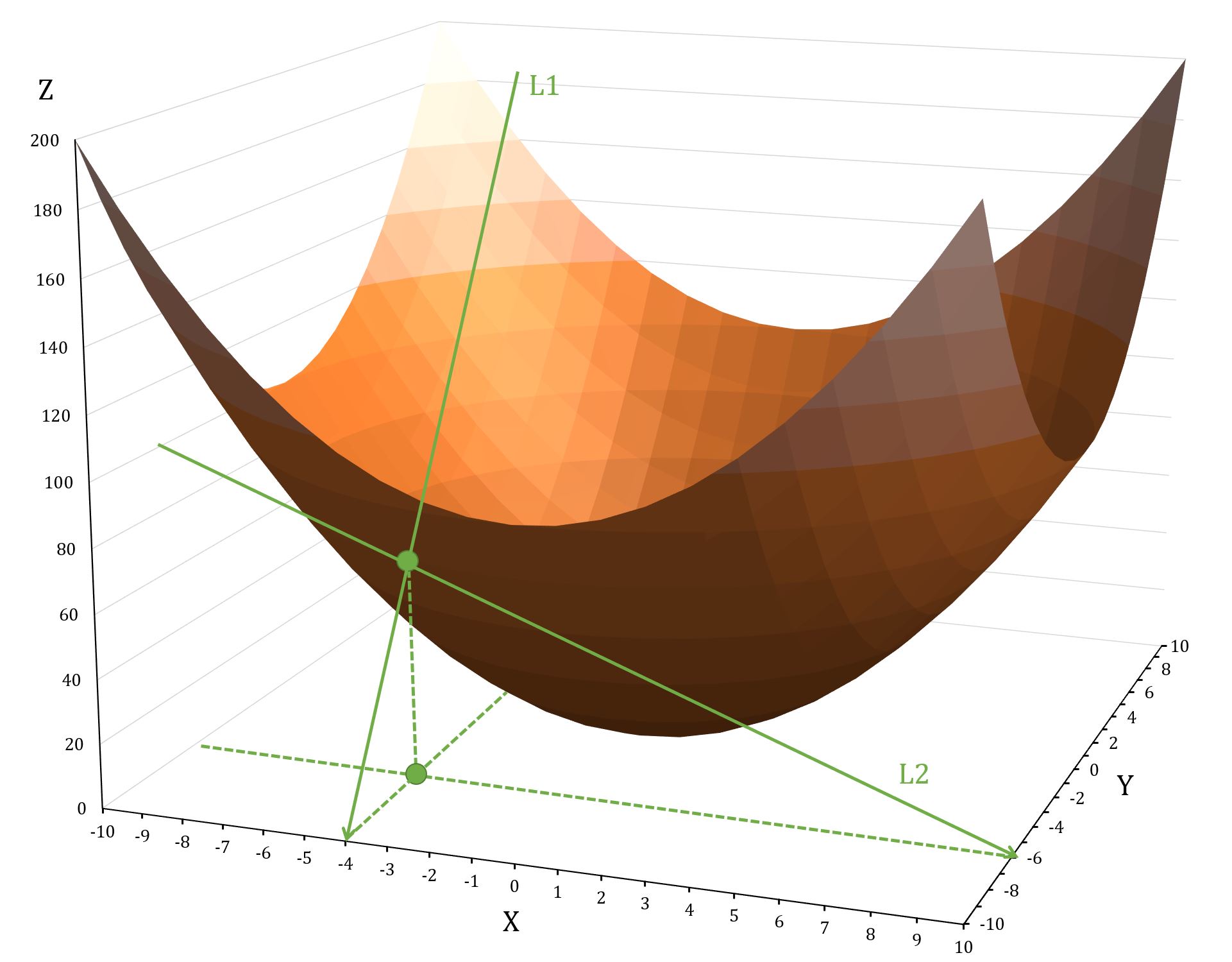
$L1$ shows how the function changes as you move along the Y-axis, while keeping $x$ constant; $L2$ shows how the function changes as you move along the X-axis, while keeping $y$ constant.

Directional Derivative

Partial derivative of a function tells about the output changes when moving slightly in the directions of axes. But when we move in a direction that is not parallel to either of the axes, the concept of directional derivative becomes crucial.

The directional derivative is mathematically expressed as the dot product of the vector $\nabla f$ composed of all partial derivatives of the function with the unit vector $\overrightarrow{w}$ which indicates the direction of the change:

where $|\overrightarrow{w}|=1$, $\theta$ is the angle between the two vectors, and

Gradient

The gradient is the direction where the output of a function has the steepest ascent. That is equivalent to finding the maximum directional derivative. This occurs when angle $\theta$ between the vectors $\nabla f$ and $\overrightarrow{w}$ is $0$, as $\cos 0=1$, implying that $\overrightarrow{w}$ aligns with the direction of $\nabla f$. $\nabla f$ is thus called the gradient of a function.

Naturally, the negative gradient points in the direction of the steepest descent.

Chain Rule

The chain rule describes how to calculate the derivative of a composite function. In the simpliest form, the derivative of a composite function $f(g(x))$ can be calculated by multiplying the derivative of $f$ with respect to $g$ by the derivative of $g$ with respect to $x$:

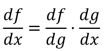
For example, $s(x)={(2x+1)}^2$ is composed of $s(u)=u^2$ and $u(x)=2x+1$:

In a multi-variable composite function, the partial derivatives are obtained by applying the chain rule to each variable.

For example, $s(x,y)=(2x+\mathrm{y})(y-3)$ is composed of $s(f,g)=fg$ and $f(x,y)=2x+\mathrm{y}$ and $g(x,y)=y-3$: