Results Visualization

The Results Pane displays the results of the executed query.

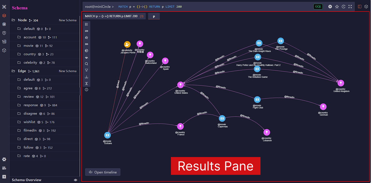
Interactive Overlays

Interactive overlays on the Results Pane include:

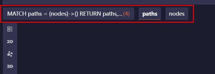
• The top displays the query history and returned alias tabs. You can click a query history to switch back to its results.

• The left side offers a set of tools to interact with the graph:

• The bottom-left corner has an Open timeline option to visualize how the data evolves over time. Learn more about timeline

Layouts

The layout of a graph visualization refers to how nodes are positioned, and edges are routed within the graph. Each layout has distinct characteristics that can help convey different aspects of the data. Ultipa Manager provides the following layouts for visualizing graphs in the 2D view:

Force-directed: This layout simulates physical forces—nodes repel each other while edges pull connected nodes together—until a balanced state is reached. It reveals community structures in the graph. However, its iterative nature makes it computationally intensive, especially for large graphs.

Tree: This layout is designed for tree structures, organizing nodes in a hierarchical, branching pattern. It supports non-layered arrangements, making it ideal for displaying clear parent-child relationships. While efficient and easy to read, it is limited to acyclic graphs without shared children.

Dagre: This layout is tailored for Directed Acyclic Graphs (DAGs) and arranges nodes in layered ranks to emphasize flow direction. It minimizes edge crossings to improve readability, making it well-suited for workflows, dependency graphs, and other structured, directional data.

Eclipse Layout Kernel (ELK): This is a flexible layout engine that supports multiple strategies, including layered (like Dagre), orthogonal, force-directed, and tree-based layouts. It is well-suited for large, complex graphs where layout customization, advanced edge routing, and fine-tuned control are required.

Circular: This layout arranges all nodes evenly along the circumference of a circle, with edges drawn as straight lines between them. It provides a symmetrical view that highlights central or highly connected nodes but can become visually cluttered as graph size and edge density increase.

Style

In the Graph view, you can apply styles to nodes and edges, customizing their color, size, shape, and text labels for better clarity and emphasis.

NOTE

Styles created by different users in the same database are shared.

NOTE

If no custom style is applied, a default style is used, which assigns distinct colors to nodes and edges based on their respective schemas.

Apply a Style

You can apply a style by selecting its checkbox:

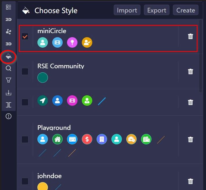
Create a Style

Click Style > Create to define a new style. You may optionally name the style and add node and edge styles.

For each node or edge style, you can specify the applicable schemas and properties. Then,

• Basic Style allows you to configure shape, size, color, and label for nodes or edges.
• Advanced Style enables dynamic styling by setting color or size ranges based on the values of a numeric property.

NOTE

If you choose Image or Circular Image as the node shape, make sure the image URLs are stored in the specified node property.

If multiple node or edge styles are added, those listed lower in the order take precedence over those above. You can adjust the order by dragging and dropping the corresponding style cards.

Import/Export Styles

Click Style > Export to export all styles as a .txt file. You can import this file into another database to transfer or back up style configurations.

Canvas Operations

The canvas that displays the query results supports various operations for interacting with the graph:

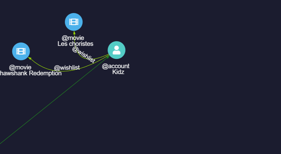
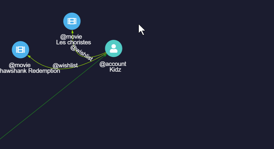
Hover Over Nodes and Edges

Hover over a node or an edge to view its schema and properties:

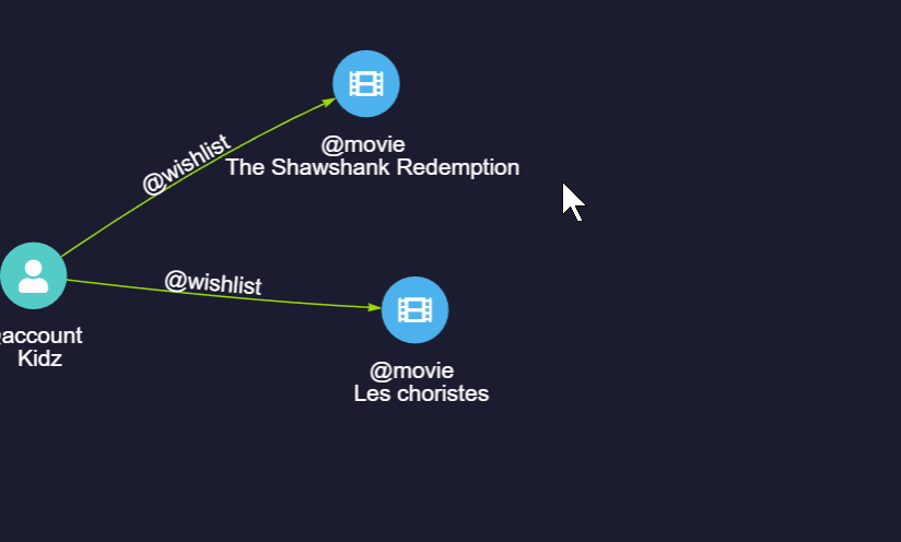
Select a Node

Select (left-click) a node to access options for spreading from it:

• Click Select Neighbors to choose one or more direct neighbors to include in the spread.
• Click an option under Spread by to spread from the node through specific edge schema and direction to certain node schema.

Right-Click a Node

Right-click a node to open a menu with the following options:

• Edit: Edit the node.
• Delete: Delete the node along with all its connected edges.
• Hide: Hide the node along with all its connected edges.
• Lock/Unlock: Lock or unlock the position of the node in the canvas.
• Add Edge: Add a new edge from this node.
• Search More: Spread from the node with the specified depth, direction, and other conditions.

Select an Edge

Select (left-click) an edge to access the following options:

• Edit: Edit the edge.
• Delete: Delete the edge.

Canvas Menu

Right-click empty area on the canvas to open the canvas menu with the following options:

• Add Node: Add a new node.
• Lock/Unlock All: Lock or unlock the positions of all nodes in the canvas.
• Collapse/Expand Edges: Collapse or expand the multiple edges exist between any two nodes.
• Collapse/Expand Nodes: Hold the Ctrl key to select multiple nodes in the canvas and collapse them into a single representation. Click Expand Nodes to restore the original individual nodes.
• Search More: Spread from selected nodes in the canvas with specified depth, direction, and other conditions.

Timeline

When NODE or PATH results include nodes or edges with properties of the timestamp or datetime type, the Open timeline button becomes available at the bottom-left of the canvas in the Graph view. This feature allows you to visualize how your data evolves over time.

The timeline range is determined by the minimum and maximum values of the properties selected under Settings > Select time properties. By default, the full range is selected, but you can adjust it by dragging the two handles. The selected slice filters the canvas to show only data whose properties fall within that range. Click Play to automatically move the slice across the timeline; the playback speed is controlled by the Settings > Playback Duration.

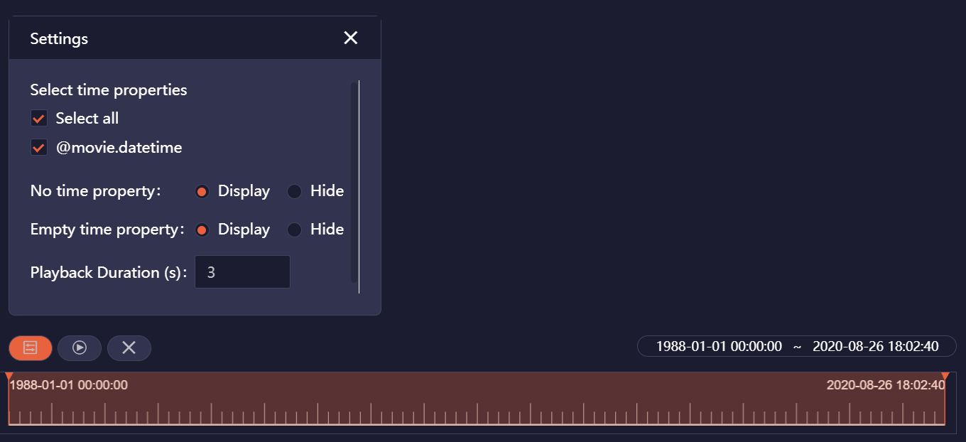
Meanwhile, you have the option to display or hide nodes and edges with No time property and Empty time property under Settings.