Result Pane

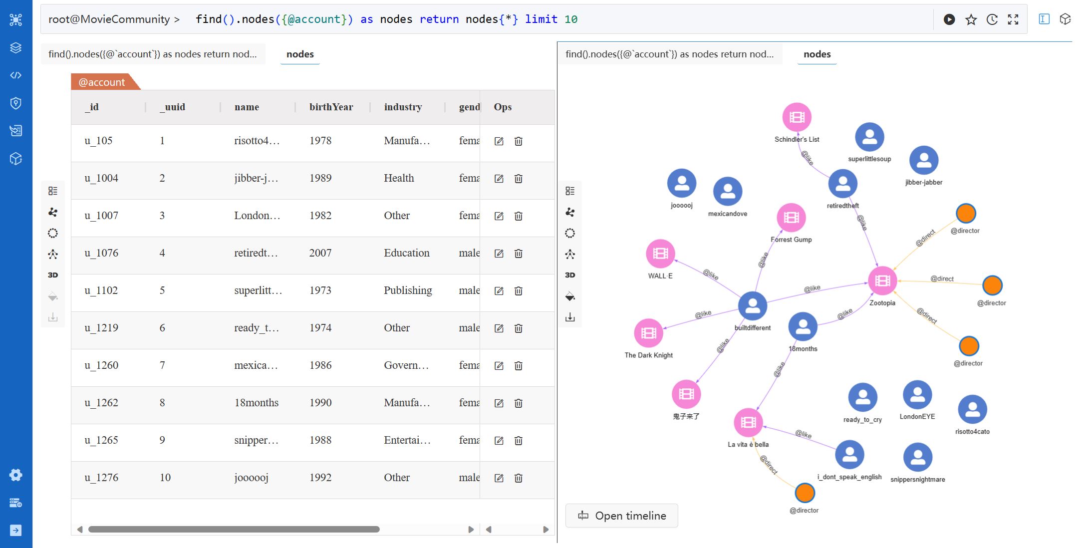
The Result Pane displays the Welcome message by default and shows the results after executing any UQL or widget.

Tools

The result pane can be split into multiple screens. Each screen contains a Tools menu placed on the left side:

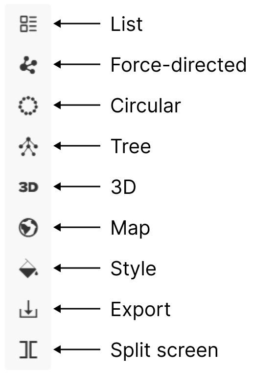
List

Click the List icon to display results in table(s).

NOTE

The List view is used by default for the NODE, EDGE, TABLE, and ATTR results. The TABLE and ATTR results can only be displayed in the List view. Learn more about the types of results

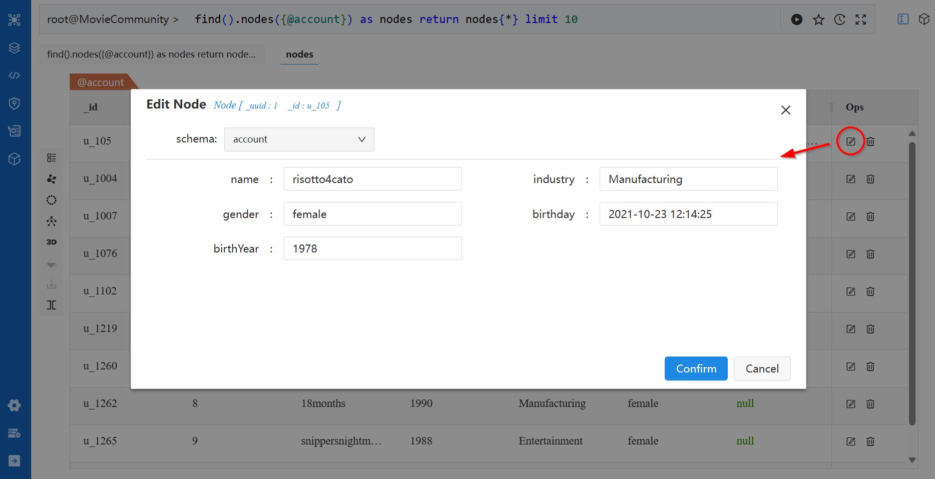
For the NODE, EDGE and PATH results, the List view provides options to Edit or Delete the nodes and edges. The TABLE and ATTR results are not editable.

The edit and delete options are available in the Ops column of the node/edge list:

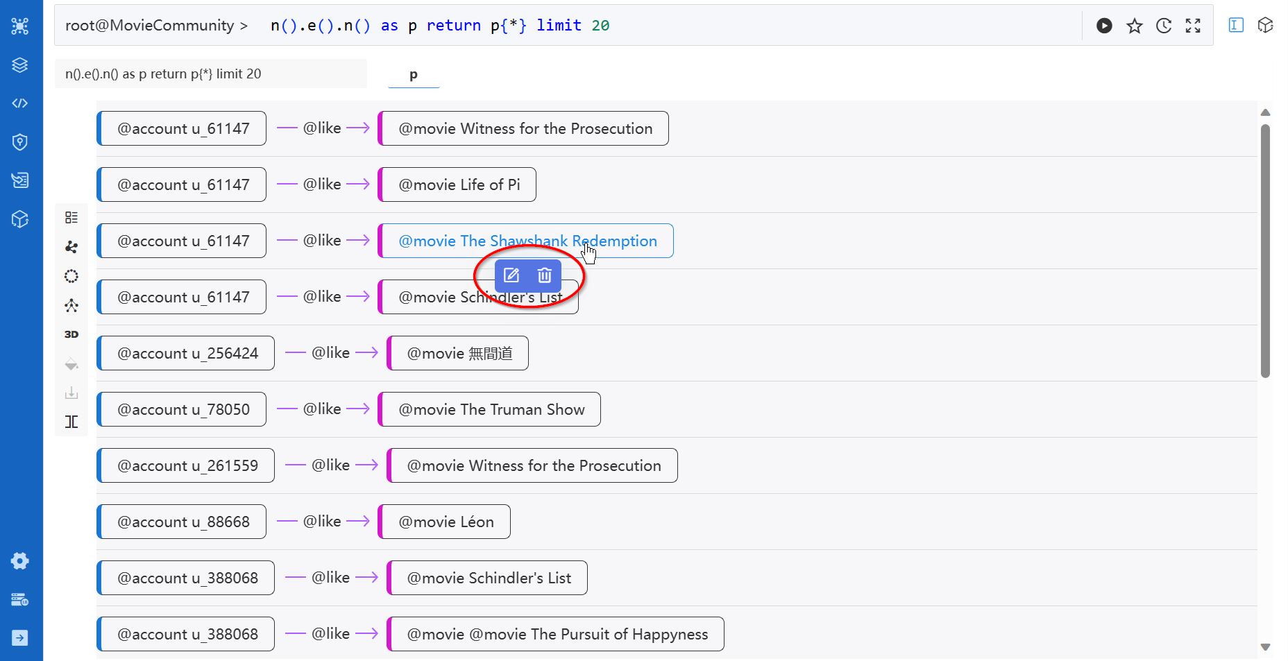
The edit and delete options appear upon clicking the node/edge label in the path list:

Force-directed / Circular / Tree

Click the Force-directed, Circular, or Tree icon to display results as a graph in the force-directed, circular, or tree layout.

Force-directed. In this layout, nodes have repulsive forces to each other to maintain spacing and prevent overlapping; while edges act as attractive forces, pulling connected nodes closer. Force-directed layout iteratively finds a balanced state, resulting in a visually pleasing arrangement of the graph.

The force directed layout naturally reveals the community or cluster structure of the graph by connections. However, it can be computationally expensive, especially for large graphs, due to its iterative nature.

Circular. The circular layout places all nodes evenly in a circular ring, with edges drawn as straight lines connecting the nodes.

The circular layout allows for easy identification of central nodes that have dense connections. However, as the number of nodes and edges increases, the circular arrangement may become crowded, making it difficult to maintain clarity and avoid overlapping elements.

Tree. The tree layout puts a node at the top as root, with its neighbor nodes branching out layer by layer.

The tree layout effectively represents hierarchical structures, it is ideal for visualizing tree-like data. However, since the root node is determined by the longest path in the query results, some rearrangements might be needed for specific contexts.

NOTE

The Force-directed layout is used by default for the PATH results containing 200 nodes for fewer. Only the NODE and PATH results can be displayed in the Force-directed, Circular, and Tree layouts. Learn more about the types of results

Operations on Nodes

1. Hover. View the schema and all properties of a node by hovering over it:

2. Left-click. Left-click on a node brings up a circular menu with three options:

• Spread: Spread from the node. This is equivalent to executing the query spread().src(<node>).depth(<N>) limit <M>, where the <N> and <M> are set in the Depth and Limit in Settings accordingly.
• Edit: Edit the node.
• Delete: Delete the node.

3. Right-click. Right-click on a node brings up a menu with the options:

• Hide: Hide the node and all edges adjacent to it in the view.
• Lock/Unlock: In the Force-directed layout, when dragging and moving a node, other nodes also move accordingly. This option can lock/unlock the location of the node in the canvas.
• Add Edge: Add a new edge from this node.
• Search More: Spread from the node with more configurations (Depth, Direction, Filter Node, Filter Edge, Return Limit).

Operations on Edge

1. Hover. View the schema and all properties of an edge by hovering over it:

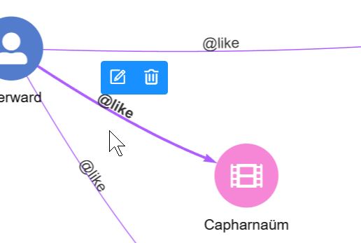
2. Left-click. Left-click on an edge brings up a menu with two options:

• Edit: Edit the edge.
• Delete: Delete the edge.

Canvas Menu

Right-Click. Right-click on any empty area in the canvas brings up a menu with the options:

• Add Node: Add a new node.
• Lock All/Unlock All: In the Force-directed layout, when dragging and moving a node, other nodes also move accordingly. This option can lock/unlock the location of all nodes in the canvas.
• Tree Layout/Circular Layout: Switch to the Tree/Circular view.
• Collapse Edges/Expand Edges: Collapse/Expand the multiple edges between any two nodes.
• Search More: Spread from nodes with some configurations (From, Depth, Direction, Filter Node, Filter Edge, Return Limit).

3D

Click the 3D icon to display results as a graph in a 3D space.

NOTE

The 3D layout is used by default for the PATH results containing more than 200 nodes. Only the NODE and PATH results can be displayed in the 3D layout. Learn more about the types of results

The 3D layout adds depth and spatial positioning to nodes and edges, reducing overlaps compared to 2D layouts. You can interact with the 3D layout by rotating, zooming, and navigating the graph from different perspectives.

However, it's important to note that the perspective and foreshortening effects in the 3D layout may distort the perceived size and distance of nodes. You should be mindful of these distortions when interpreting the layout.

In the 3D layout, the style applied to nodes and edges in 2D layouts are simplified. The same applies to the operations on nodes, edges, and the canvas.

Map

When the NODE or PATH results contain nodes with properties of the point type, the Map view becomes available to display data on a map:

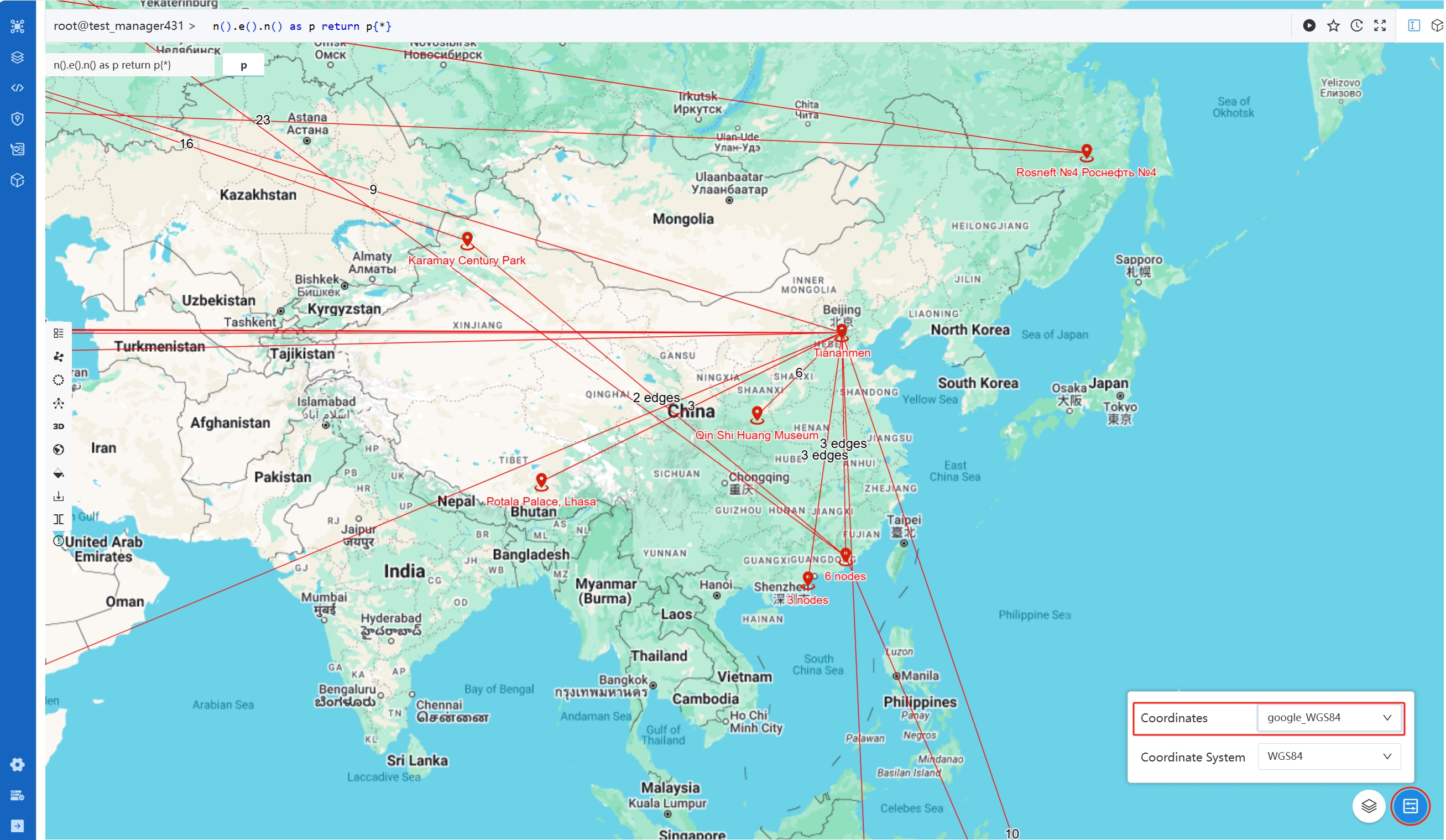
You can specify the point property, the coordinate system, and the map by clicking the settings and layers icon in the bottom right corner of the map.

Style

In the Force-directed, Circular, Tree, and 3D layouts, you can apply styles to nodes and edges. This allows customization of their color, size, shape, and label based on their schema and the value of properties.

NOTE

The styles created by different users in one instance are shared.

NOTE

When no custom style is applied, a default style is used that assigns unique colors to nodes and edges based on their respective schema.

Create a Style

A style consists of one or multiple node and edge styles. For each Node Style or Edge Style, you need to:

1. Specify the target nodes or edges

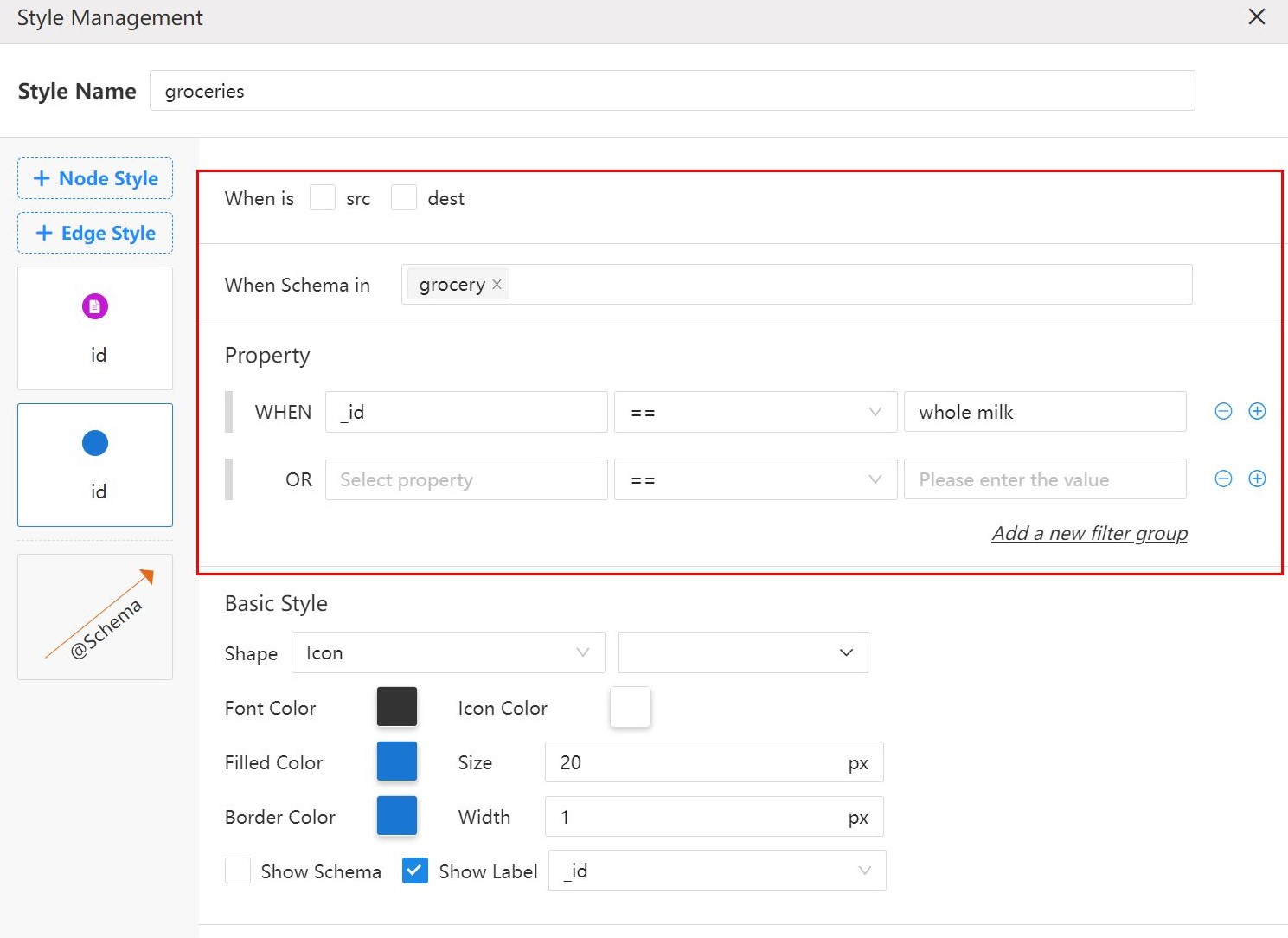
• When is src/dest: This is available for Node Style only. The style will only be applied to the start nodes (src) or end nodes (dest) of edges in the graph.
• When Schema in: The style will only be applied to nodes/edges of certain schema(s).
• Property: The style will only be applied to nodes/edges with the required property values.

2. Edit the Style

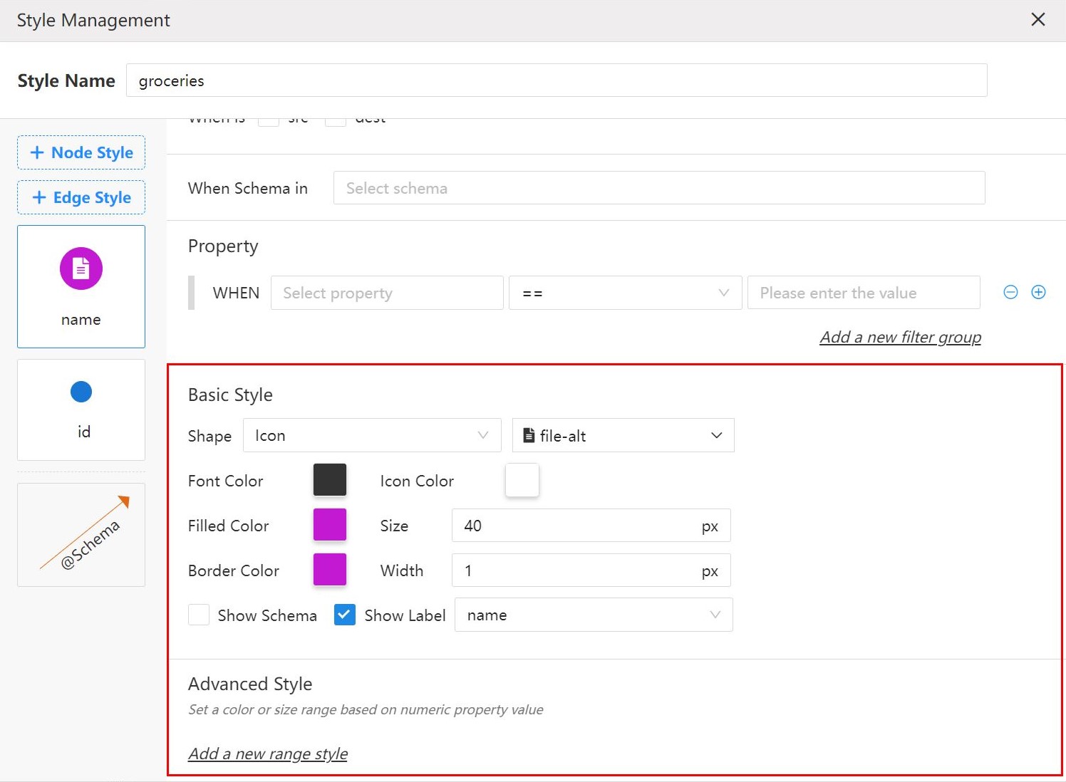
Under the Basic Style, you can edit the shape, size, color, label and so on for nodes/edges.

NOTE

If using Image or Circular Image as the shape for nodes, save the image links into the specified node property.

Under the Advanced Style, you can set the color or size range for nodes/edges based on the values of a numeric property.

3. Re-order the Style Cards

If multiple node/edge styles are created with conflicting settings for the same target nodes/edges, the node/edge style positioned lower will take precedence over those above it. You can adjust the ordering of node/edge styles by dragging and dropping the corresponding cards.

NOTE

The saved style won't be applied automatically. You need to manually select the newly created style. Sometimes you may need to re-run the corresponding UQL.

Import/Export Styles

At the top of the style list, you can export all styles in the instance as a .TXT file. This file can then be imported into any other instance, facilitating the transfer or backup of styles.

Export

You can export the results in three formats:

• JSON
• PNG: Only available in the Force-directed, Circular, Tree, and 3D layouts.
• XLSX: Only available for the NODE and EDGE results.

Split screen

Click the Split screen icon to add another screen to display the results. You can have up to two screens.

When multiple screens are present, the one with the highlighted border is considered active and will be used for the next execution. To change the active screen, simply click on any other screen.

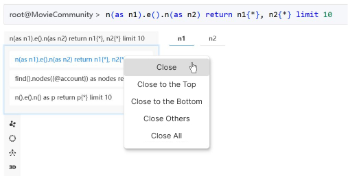
Execution History

Each result screen retains its execution history, which is located at the top left corner:

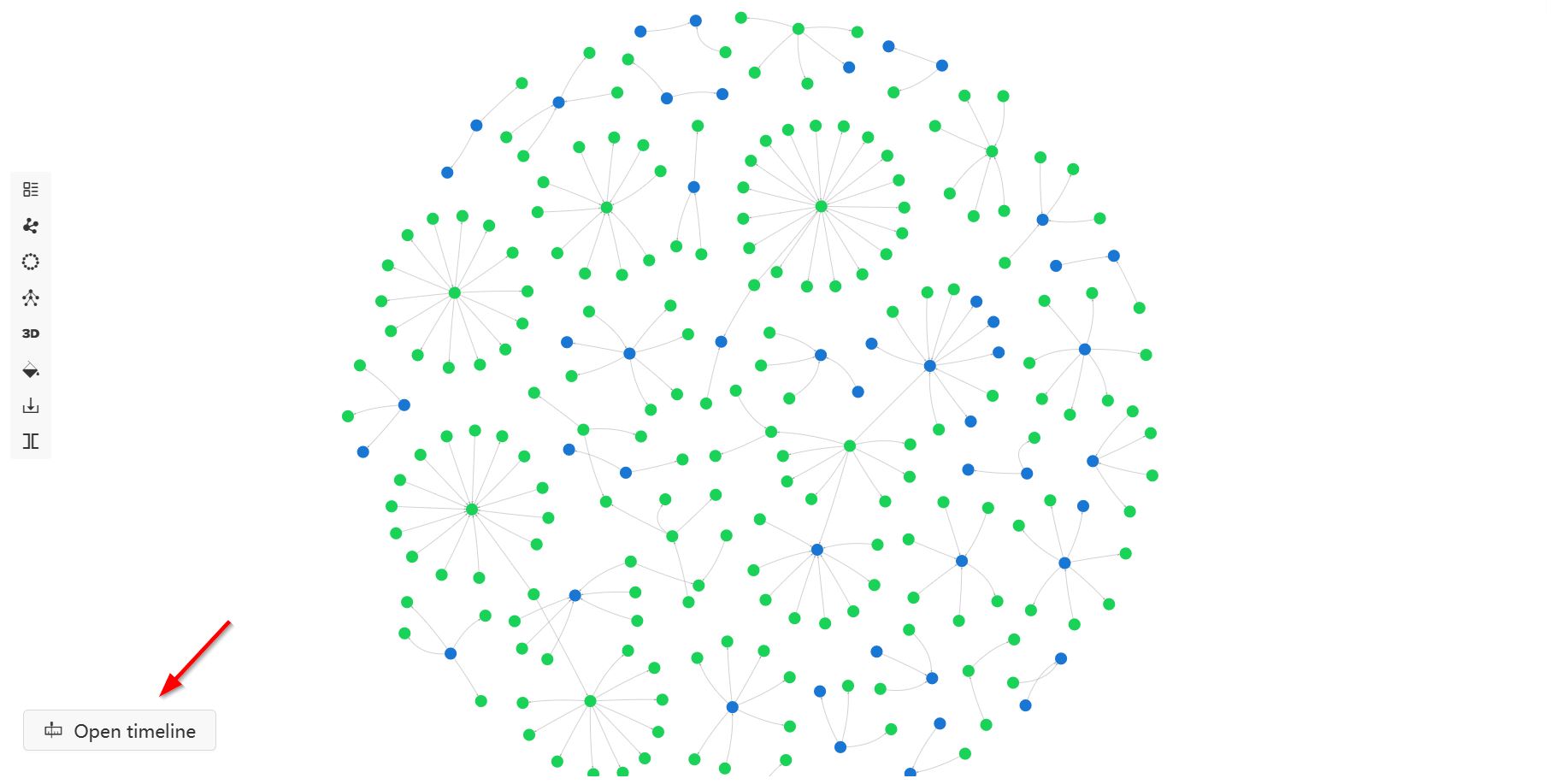
Timeline

When the NODE or PATH results contain nodes or edges with properties of the timestamp or datetime type, the Open timeline button becomes available at the bottom left of the canvas in the Force-directed, Circular, and Tree layouts. This timeline feature allows you to visualize how your data evolves over time.

The range of the entire timeline depends on the minimum and maximum values of properties selected under Settings > Select time properties. By default, the entire time range is selected, but you can adjust it to a shorter range by moving the two handles. The slice can be moved across the timeline, displaying only the data whose properties fall within that range on the canvas. Click Play to automatically progress the slice until the end of the timeline; the playback speed is determined by the Playback Duration under Settings.

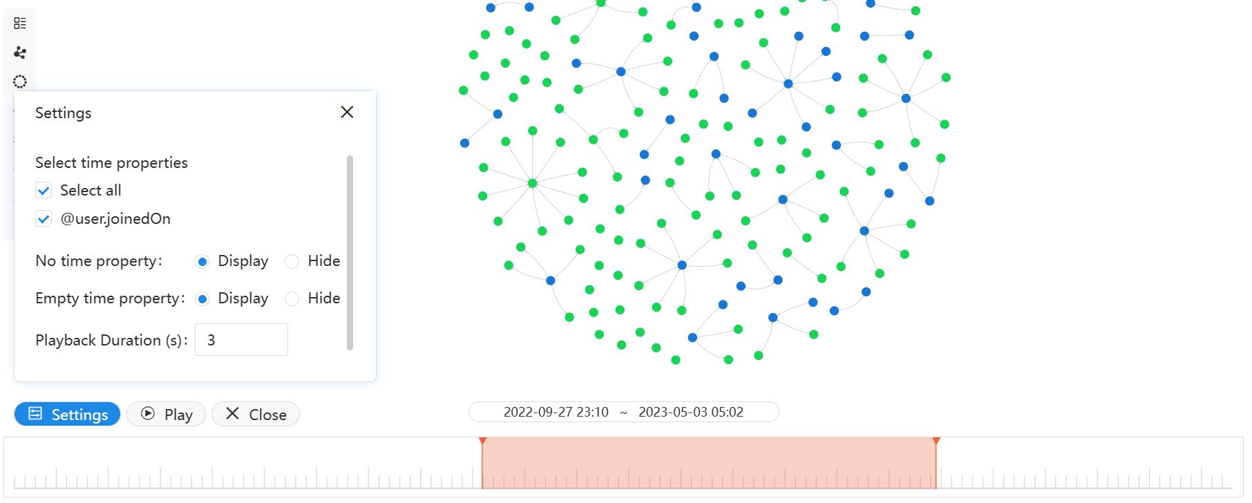
Meanwhile, you have the option to display or hide nodes and edges with No time property and Empty time property under Settings.